The ACCESS-NRI Evaluation Frameworks

Overview

Teaching: 20 min
Exercises: 30 min
Compatibility:

Questions

• What are the ACCESS-NRI supported evaluation frameworks?

• How do I get started?

• Where can I find help?

Objectives

The Model Evaluation and Diagnostics (MED) Team is Here to Help!

We support infrastructure (software + data) and provide technical support / training to the ACCESS community.

• Tool Deployment on NCI Gadi: We make sure essential tools like ESMValTool and ILAMB are ready to go on NCI Gadi, so your research workflows run smoothly.

• Evaluation Tools & Recipes: We develop, support, and fine-tune evaluation tools and scripts, ensuring they’re up to scratch.

• Publication & Dissemination: Need to get your work out there? We assist with publishing and sharing your evaluation scripts.

• Training: Whether you’re a newbie or a pro, we offer training for all levels to help you make the most of our tools and resources.

• Community Hub: We’re your go-to for collaboration and knowledge-sharing, keeping the ACCESS ecosystem thriving.

If you need support, the MED team is here to help!

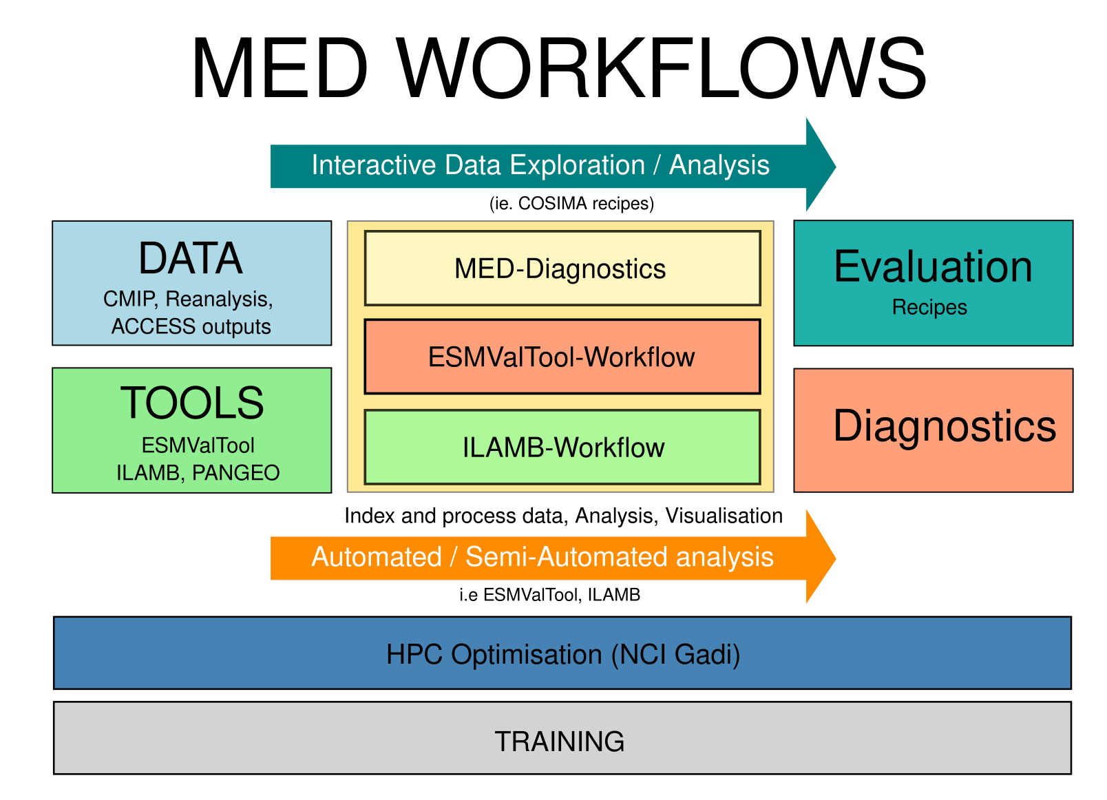
ACCESS-NRI Evaluation tools and infrastructure

Here is the current list of tools and supporting infrastructure under the ACCESS-NRI Model Evaluation and Diagnostics team responsibility:

• MED Conda Environments
• ESMValTool-Workflow
• ILAMB-Workflow
• ACCESS MED Diagnostics
• ACCESS-NRI Intake catalogue
• ACCESS-NRI Data Replicas for Model Evaluation and Diagnostics

MED Conda Environments

To ensure effective and efficient evaluation of model outputs, it is crucial to have a well-maintained and reliable analysis environment on the NCI Gadi supercomputer. Our approach involves releasing tools within containerized Conda environments, providing a consistent and dependable platform for users. These containerized environments simplify the deployment process, ensuring that all necessary dependencies and configurations are included, which minimizes setup time and potential issues.

ESMValTool-Workflow

ESMValTool-workflow is the ACCESS-NRI software and data infrastructure that enables the ESMValTool evaluation framework on NCI Gadi. It includes:

• The ESMValCore Python packages: This core library is designed to facilitate the preprocessing of climate data, offering a structured and efficient way to handle complex datasets.
• The ESMValTool collection of recipes, diagnostics and observation CMORisers.
• A data pool of CMORised observational datasets.

ESMValTool-workflow is configured to use the existing NCI supported CMIP data collections.

ESMValTool meets the community’s need for a robust, reliable, and reproducible framework to evaluate ACCESS climate models. Specifically developed with CMIP evaluation in mind, the software is well-suited for this purpose.

How do I get started?

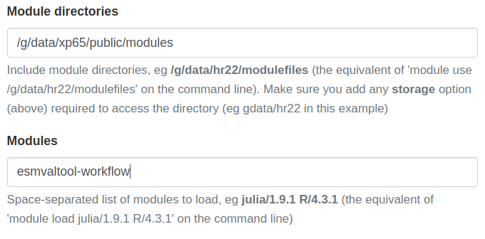
The ESMValCore and ESMValTool python tools and their dependencies are deployed on Gadi within an ESMValTool-workflow containerized Conda environment that can be loaded as a module.

Using the command line and PBS jobs

If you have carefully completed the requirements, you should already be a member of the xp65 project and be ready to go.

module use /g/data/xp65/public/modules
# Load the ESMValTool-Workflow:
module load esmvaltool-workflow

Using ARE

If you have carefully completed the requirements, you should already be a member of the xp65 project and be ready to go.

ILAMB-Workflow

The International Land Model Benchmarking (ILAMB) project is a model-data intercomparison and integration project designed to improve the performance of land models and, in parallel, improve the design of new measurement campaigns to reduce uncertainties associated with key land surface processes.

The ACCESS-NRI Model Evaluation and Diagnostics team is releasing and supporting NCI configuration of ILAMB under the name ILAMB-workflow.

ILAMB-workflow is the ACCESS-NRI software and data infrastructure that enables the ILAMB evaluation framework on NCI Gadi. It includes:

• the ILAMB Python packages
• a series of ILAMB outputs for ACCESS model evaluation and
• the ILAMB-Data collection of observational datasets.

ILAMB-workflow is configured to use the existing NCI supported CMIP data collections.

ILAMB addresses the needs of the Land community for a robust, reliable, and reproducible framework for evaluating land surface models.

How do I get started?

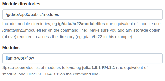
The ILAMB python tool and its dependencies are deployed on Gadi within an ILAMB-workflow containerized Conda environment that can be loaded as a module.

Using the command line and PBS jobs

If you have carefully completed the requirements, you should already be a member of the xp65 project and be ready to go.

module use /g/data/xp65/public/modules
# Load the ILAMB-Workflow:
module load ilamb-workflow

Using ARE

If you have carefully completed the requirements, you should already be a member of the xp65 project and be ready to go.

Key Points

Introducing ESMValTool

Overview

Teaching: 5 min
Exercises: 10 min
Compatibility:

Questions

• What is ESMValTool?

• Who are the people behind ESMValTool?

Objectives

• Familiarize with ESMValTool

• Synchronize expectations

What is ESMValTool?

This tutorial is a first introduction to ESMValTool. Before diving into the technical steps, let’s talk about what ESMValTool is all about.

What is ESMValTool?

What do you already know about or expect from ESMValTool?

ESMValTool is…

EMSValTool is many things, but in this tutorial we will focus on the following traits:

✓ A Python-based preprocessing framework

✓ A Standardised framework for climate data analysis

✓ A collection of diagnostics for reproducible climate science

✓ A community effort

A Python-based preprocessing framework

ESMValTool is powered by ESMValCore, a powerfull python-based workflow engine that facilitates CMIP analysis. ESMValCore implements the core functionality of ESMValTool: it takes care of finding, opening, checking, fixing, concatenating, and preprocessing CMIP data and several other supported datasets. ESMValCore has matured as a reliable foundation for the ESMValTool with recent addition making it attractive as a lightweight approach to CMIP evaluation.

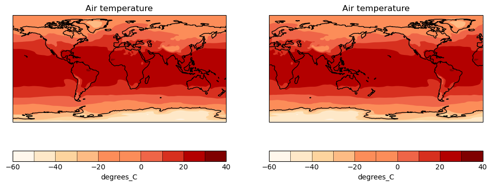
A common scenario consist in visualising the global temperature of an historical run over a 2 year period. To do so, you need first to:

• Find the data
• Extract the period of interest
• Calculate the mean
• Convert the units to degrees celsius
• Finally Plot the data

The following example illustrate how to leverage ESMValCore, the engine powering the ESMValTool collection of recipes, to quickly load CMIP data and do some analysis on them.

 from esmvalcore.dataset import Dataset
 from esmvalcore.preprocessor import extract_time
 from esmvalcore.preprocessor import climate_statistics
 from esmvalcore.preprocessor import convert_units

 dataset = Dataset(
   short_name='tas',
   project='CMIP6',
   mip="Amon",
   exp="historical",
   ensemble="r1i1p1f1",
   dataset='ACCESS-ESM1-5',
   grid="gn"
)

 temperature = dataset.load()
 temperature_1990_1991 = extract_time(temperature, start_year=1990, start_month=1, start_day=1, end_year=1991, end_month=1, end_day=1) 
 temperature_weighted_mean = climate_statistics(temperature_1990_1991, operator="mean")
 temperature_celsius = convert_units(temperature_weighted_mean, units="degrees_C")

Example Plots

ESMValCore uses Iris Cube to manipulate data. Iris can thus be used to quickly plot the data in a notebook, but you could use your package of choice.

 import cartopy.crs as ccrs
 import matplotlib.pyplot as plt
 from matplotlib import colormaps
 
 import iris
 import iris.plot as iplt
 import iris.quickplot as qplt
 
 # Load a Cynthia Brewer palette.
 brewer_cmap = colormaps["brewer_OrRd_09"]
 
 # Create a figure
 plt.figure(figsize=(12, 5))
 
 # Plot #1: countourf with axes longitude from -180 to 180
 proj = ccrs.PlateCarree(central_longitude=0.0)
 plt.subplot(121, projection=proj)
 qplt.contourf(temperature_weighted_mean, brewer_cmap.N, cmap=brewer_cmap)
 plt.gca().coastlines()
 
 # Plot #2: contourf with axes longitude from 0 to 360
 proj = ccrs.PlateCarree(central_longitude=-180.0)
 plt.subplot(122, projection=proj)
 qplt.contourf(temperature_weighted_mean, brewer_cmap.N, cmap=brewer_cmap)
 plt.gca().coastlines()
 iplt.show()

Exercises

ESMValCore has a growing collection of preprocessors, have a look at the documentation and see what is available.

• Open an ARE session and run the above example.
• See if you can load other datasets
• change the time period
• Add a new preprocessing step

A Standardised framework for climate data analysis

ESMValTool is a software project that was designed by and for climate scientists to evaluate CMIP data in a standardized and reproducible manner.

The central component of ESMValTool that we will see in this tutorial is the recipe. Any ESMValTool recipe is basically a set of instructions to reproduce a certain result. The basic structure of a recipe is as follows:

• Documentation with relevant (citation) information
• Datasets that should be analysed
• Preprocessor steps that must be applied
• Diagnostic scripts performing more specific evaluation steps

An example recipe could look like this:

documentation:
  title: This is an example recipe.
  description: Example recipe
  authors:
    - lastname_firstname

datasets:
  - {dataset: ACCESS-CM2, project: CMIP6, exp: historical, mip: Amon, 
     ensemble: r1i1p1f1, start_year: 1960, end_year: 2005}

preprocessors:
  global_mean:
    area_statistics:
      operator: mean

diagnostics:
  average_plot:
    description: plot of global mean temperature change
    variables:
      temperature:
        short_name: tas
        preprocessor: global_mean
    scripts: examples/diagnostic.py

Understanding the different section of the recipe

Try to figure out the meaning of the different dataset keys. Hint: they can be found in the documentation of ESMValTool.

Solution

The keys are explained in the ESMValTool documentation, in the Recipe section , under datasets

A collection of diagnostics for reproducible climate science

More than a tool, ESMValTool is a collection of publicly available recipes and diagnostic scripts. This makes it possible to easily reproduce important results.

Explore the available recipes

Go to the ESMValTool Documentation webpage and explore the Available recipes section. Which recipe(s) would you like to try?

A community effort

ESMValTool is built and maintained by an active community of scientists and software engineers. It is an open source project to which anyone can contribute. Many of the interactions take place on GitHub. Here, we briefly introduce you to some of the most important pages.

Meet the ESMValGroup

Go to github.com/ESMValGroup. This is the GitHub page of our ‘organization’. Have a look around. How many collaborators are there? Do you know any of them?

Near the top of the page there are 2 pinned repositories: ESMValTool and ESMValCore. Visit each of the repositories. How many people have contributed to each of them? Can you also find out how many people have contributed to this tutorial?

Issues and pull requests

Go back to the repository pages of ESMValTool or ESMValCore. There are tabs for ‘issues’ and ‘pull requests’. You can use the labels to navigate them a bit more. How many open issues are about enhancements of ESMValTool? And how many bugs have been fixed in ESMValCore? There is also an ‘insights’ tab, where you can see a summary of recent activity. How many issues have been opened and closed in the past month?

Conclusion

This concludes the introduction of the tutorial. You now have a basic knowledge of ESMValTool and its community. The following episodes will walk you through the installation, configuration and running your first recipes.

Key Points

• ESMValTool provides a reliable interface to analyse and evaluate climate data

• A large collection of recipes and diagnostic scripts is already available

• ESMValTool is built and maintained by an active community of scientists and developers

Running your first recipe

Overview

Teaching: 15 min
Exercises: 15 min
Compatibility:

Questions

• How to run a recipe?

• What happens when I run a recipe?

Objectives

• Run an existing ESMValTool recipe

• Examine the log information

• Navigate the output created by ESMValTool

• Make small adjustments to an existing recipe

This episode describes how ESMValTool recipes work, how to run a recipe and how to explore the recipe output. By the end of this episode, you should be able to run your first recipe, look at the recipe output, and make small modifications.

Import module in GADI

You may want to open VS Code with a remote SSH connection to Gadi and use the VS Code terminal, then you can later view the recipe file. Refer to VS Code setup.

In a terminal with an SSH connection into Gadi, load the module to use ESMValTool on Gadi.

module use /g/data/xp65/public/modules
module load esmvaltool-workflow

Running an existing recipe

The recipe format has briefly been introduced in the Introduction episode. To see all the recipes that are shipped with ESMValTool, type

esmvaltool recipes list

We will start by running examples/recipe_python.yml. This is the command with ESMValTool installed.

esmvaltool run examples/recipe_python.yml

On Gadi, this can be done using the esmvaltool-workflow wrapper in the loaded module.

esmvaltool-workflow run examples/recipe_python.yml

or if you have the user configuration file in your current directory then

esmvaltool-workflow run --config_file ./config-user.yml examples/recipe_python.yml

You should see that Gadi has created a PBS job to run the recipe. You can check your queue status with qstat.

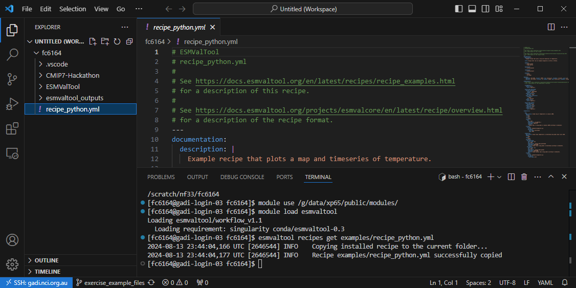
[fc6164@gadi-login-01 fc6164]$ module load esmvaltool
Welcome to the ACCESS-NRI ESMValTool-Workflow

enter command `esmvaltool-workflow` for help

Loading esmvaltool/workflow_v1.2
  Loading requirement: singularity conda/esmvaltool-0.4

[fc6164@gadi-login-01 fc6164]$ esmvaltool-workflow run recipe_python.yml 
conda/esmvaltool-0.4
123732363.gadi-pbs
Running recipe: recipe_python.yml

[fc6164@gadi-login-01 fc6164]$ qstat
Job id                 Name             User              Time Use S Queue
---------------------  ---------------- ----------------  -------- - -----
123732363.gadi-pbs     recipe_python    fc6164                   0 Q normal-exec     
[fc6164@gadi-login-01 fc6164]$ 

If everything is okay, the final log message should be “Run was successful”. The exact output varies depending on your machine, this is an example of a successful log output below.

Example output

2024-05-15 07:04:08,041 UTC [134535] INFO    
______________________________________________________________________
         _____ ____  __  ____     __    _ _____           _
        | ____/ ___||  \/  \ \   / /_ _| |_   _|__   ___ | |
        |  _| \___ \| |\/| |\ \ / / _` | | | |/ _ \ / _ \| |
        | |___ ___) | |  | | \ V / (_| | | | | (_) | (_) | |
        |_____|____/|_|  |_|  \_/ \__,_|_| |_|\___/ \___/|_|
______________________________________________________________________

ESMValTool - Earth System Model Evaluation Tool.

http://www.esmvaltool.org

CORE DEVELOPMENT TEAM AND CONTACTS:
 Birgit Hassler (Co-PI; DLR, Germany - birgit.hassler@dlr.de)
 Alistair Sellar (Co-PI; Met Office, UK - alistair.sellar@metoffice.gov.uk)
 Bouwe Andela (Netherlands eScience Center, The Netherlands - b.andela@esciencecenter.nl)
 Lee de Mora (PML, UK - ledm@pml.ac.uk)
 Niels Drost (Netherlands eScience Center, The Netherlands - n.drost@esciencecenter.nl)
 Veronika Eyring (DLR, Germany - veronika.eyring@dlr.de)
 Bettina Gier (UBremen, Germany - gier@uni-bremen.de)
 Remi Kazeroni (DLR, Germany - remi.kazeroni@dlr.de)
 Nikolay Koldunov (AWI, Germany - nikolay.koldunov@awi.de)
 Axel Lauer (DLR, Germany - axel.lauer@dlr.de)
 Saskia Loosveldt-Tomas (BSC, Spain - saskia.loosveldt@bsc.es)
 Ruth Lorenz (ETH Zurich, Switzerland - ruth.lorenz@env.ethz.ch)
 Benjamin Mueller (LMU, Germany - b.mueller@iggf.geo.uni-muenchen.de)
 Valeriu Predoi (URead, UK - valeriu.predoi@ncas.ac.uk)
 Mattia Righi (DLR, Germany - mattia.righi@dlr.de)
 Manuel Schlund (DLR, Germany - manuel.schlund@dlr.de)
 Breixo Solino Fernandez (DLR, Germany - breixo.solinofernandez@dlr.de)
 Javier Vegas-Regidor (BSC, Spain - javier.vegas@bsc.es)
 Klaus Zimmermann (SMHI, Sweden - klaus.zimmermann@smhi.se)

For further help, please read the documentation at
http://docs.esmvaltool.org. Have fun!

2024-05-15 07:04:08,044 UTC [134535] INFO    Package versions
2024-05-15 07:04:08,044 UTC [134535] INFO    ----------------
2024-05-15 07:04:08,044 UTC [134535] INFO    ESMValCore: 2.10.0
2024-05-15 07:04:08,044 UTC [134535] INFO    ESMValTool: 2.10.0
2024-05-15 07:04:08,044 UTC [134535] INFO    ----------------
2024-05-15 07:04:08,044 UTC [134535] INFO    Using config file /pfs/lustrep1/users/username/esmvaltool_tutorial/config-user.yml
2024-05-15 07:04:08,044 UTC [134535] INFO    Writing program log files to:
/users/username/esmvaltool_tutorial/esmvaltool_output/recipe_python_20240515_070408/run/main_log.txt
/users/username/esmvaltool_tutorial/esmvaltool_output/recipe_python_20240515_070408/run/main_log_debug.txt
2024-05-15 07:04:08,503 UTC [134535] INFO    Using default ESGF configuration, configuration file /users/username/.esmvaltool/esgf-pyclient.yml not present.
2024-05-15 07:04:08,504 UTC [134535] WARNING 
ESGF credentials missing, only data that is accessible without
logging in will be available.

See https://esgf.github.io/esgf-user-support/user_guide.html
for instructions on how to create an account if you do not have
one yet.

Next, configure your system so esmvaltool can use your
credentials. This can be done using the keyring package, or
you can just enter them in /users/username/.esmvaltool/esgf-pyclient.yml.

keyring
=======
First install the keyring package (requires a supported
backend, see https://pypi.org/project/keyring/):
$ pip install keyring

Next, set your username and password by running the commands:
$ keyring set ESGF hostname
$ keyring set ESGF username
$ keyring set ESGF password

To check that you entered your credentials correctly, run:
$ keyring get ESGF hostname
$ keyring get ESGF username
$ keyring get ESGF password

configuration file
==================
You can store the hostname, username, and password or your OpenID
account in a plain text in the file /users/username/.esmvaltool/esgf-pyclient.yml like this:

logon:
 hostname: "your-hostname"
 username: "your-username"
 password: "your-password"

or your can configure an interactive log in:

logon:
 interactive: true

Note that storing your password in plain text in the configuration
file is less secure. On shared systems, make sure the permissions
of the file are set so only you can read it, i.e.

$ ls -l /users/username/.esmvaltool/esgf-pyclient.yml

shows permissions -rw-------.


2024-05-15 07:04:09,067 UTC [134535] INFO    Starting the Earth System Model Evaluation Tool at time: 2024-05-15 07:04:09 UTC
2024-05-15 07:04:09,068 UTC [134535] INFO    ----------------------------------------------------------------------
2024-05-15 07:04:09,068 UTC [134535] INFO    RECIPE   = /LUMI_TYKKY_D1Npoag/miniconda/envs/env1/lib/python3.11/site-packages/esmvaltool/recipes/examples/recipe_python.yml
2024-05-15 07:04:09,068 UTC [134535] INFO    RUNDIR     = /users/username/esmvaltool_tutorial/esmvaltool_output/recipe_python_20240515_070408/run
2024-05-15 07:04:09,069 UTC [134535] INFO    WORKDIR    = /users/username/esmvaltool_tutorial/esmvaltool_output/recipe_python_20240515_070408/work
2024-05-15 07:04:09,069 UTC [134535] INFO    PREPROCDIR = /users/username/esmvaltool_tutorial/esmvaltool_output/recipe_python_20240515_070408/preproc
2024-05-15 07:04:09,069 UTC [134535] INFO    PLOTDIR    = /users/username/esmvaltool_tutorial/esmvaltool_output/recipe_python_20240515_070408/plots
2024-05-15 07:04:09,069 UTC [134535] INFO    ----------------------------------------------------------------------
2024-05-15 07:04:09,069 UTC [134535] INFO    Running tasks using at most 256 processes
2024-05-15 07:04:09,069 UTC [134535] INFO    If your system hangs during execution, it may not have enough memory for keeping this number of tasks in memory.
2024-05-15 07:04:09,070 UTC [134535] INFO    If you experience memory problems, try reducing 'max_parallel_tasks' in your user configuration file.
2024-05-15 07:04:09,070 UTC [134535] WARNING Using the Dask basic scheduler. This may lead to slow computations and out-of-memory errors. Note that the basic scheduler may still be the best choice for preprocessor functions that are not lazy. In that case, you can safely ignore this warning. See https://docs.esmvaltool.org/projects/ESMValCore/en/latest/quickstart/configure.html#dask-distributed-configuration for more information. 
2024-05-15 07:04:09,113 UTC [134535] WARNING 'default' rootpaths '/users/username/climate_data' set in config-user.yml do not exist
2024-05-15 07:04:10,648 UTC [134535] INFO    Creating tasks from recipe
2024-05-15 07:04:10,648 UTC [134535] INFO    Creating tasks for diagnostic map
2024-05-15 07:04:10,648 UTC [134535] INFO    Creating diagnostic task map/script1
2024-05-15 07:04:10,649 UTC [134535] INFO    Creating preprocessor task map/tas
2024-05-15 07:04:10,649 UTC [134535] INFO    Creating preprocessor 'to_degrees_c' task for variable 'tas'
2024-05-15 07:04:11,066 UTC [134535] INFO    Found input files for Dataset: tas, Amon, CMIP6, BCC-ESM1, CMIP, historical, r1i1p1f1, gn, v20181214
2024-05-15 07:04:11,405 UTC [134535] INFO    Found input files for Dataset: tas, Amon, CMIP5, bcc-csm1-1, historical, r1i1p1, v1
2024-05-15 07:04:11,406 UTC [134535] INFO    PreprocessingTask map/tas created.
2024-05-15 07:04:11,406 UTC [134535] INFO    Creating tasks for diagnostic timeseries
2024-05-15 07:04:11,406 UTC [134535] INFO    Creating diagnostic task timeseries/script1
2024-05-15 07:04:11,406 UTC [134535] INFO    Creating preprocessor task timeseries/tas_amsterdam
2024-05-15 07:04:11,406 UTC [134535] INFO    Creating preprocessor 'annual_mean_amsterdam' task for variable 'tas_amsterdam'
2024-05-15 07:04:11,428 UTC [134535] INFO    Found input files for Dataset: tas, Amon, CMIP6, BCC-ESM1, CMIP, historical, r1i1p1f1, gn, v20181214
2024-05-15 07:04:11,452 UTC [134535] INFO    Found input files for Dataset: tas, Amon, CMIP5, bcc-csm1-1, historical, r1i1p1, v1
2024-05-15 07:04:11,455 UTC [134535] INFO    PreprocessingTask timeseries/tas_amsterdam created.
2024-05-15 07:04:11,455 UTC [134535] INFO    Creating preprocessor task timeseries/tas_global
2024-05-15 07:04:11,455 UTC [134535] INFO    Creating preprocessor 'annual_mean_global' task for variable 'tas_global'
2024-05-15 07:04:11,814 UTC [134535] INFO    Found input files for Dataset: tas, Amon, CMIP6, BCC-ESM1, CMIP, historical, r1i1p1f1, gn, v20181214, supplementaries: areacella, fx, 1pctCO2, v20190613
2024-05-15 07:04:12,184 UTC [134535] INFO    Found input files for Dataset: tas, Amon, CMIP5, bcc-csm1-1, historical, r1i1p1, v1, supplementaries: areacella, fx, r0i0p0
2024-05-15 07:04:12,186 UTC [134535] INFO    PreprocessingTask timeseries/tas_global created.
2024-05-15 07:04:12,187 UTC [134535] INFO    These tasks will be executed: timeseries/script1, timeseries/tas_global, map/script1, map/tas, timeseries/tas_amsterdam
2024-05-15 07:04:12,204 UTC [134535] INFO    Wrote recipe with version numbers and wildcards to:
file:///users/username/esmvaltool_tutorial/esmvaltool_output/recipe_python_20240515_070408/run/recipe_python_filled.yml
2024-05-15 07:04:12,204 UTC [134535] INFO    Will download 129.2 MB
Will download the following files:
50.85 KB	ESGFFile:CMIP6/CMIP/BCC/BCC-ESM1/1pctCO2/r1i1p1f1/fx/areacella/gn/v20190613/areacella_fx_BCC-ESM1_1pctCO2_r1i1p1f1_gn.nc on hosts ['aims3.llnl.gov', 'cmip.bcc.cma.cn', 'esgf-data04.diasjp.net', 'esgf.nci.org.au', 'esgf3.dkrz.de']
64.95 MB	ESGFFile:CMIP6/CMIP/BCC/BCC-ESM1/historical/r1i1p1f1/Amon/tas/gn/v20181214/tas_Amon_BCC-ESM1_historical_r1i1p1f1_gn_185001-201412.nc on hosts ['aims3.llnl.gov', 'cmip.bcc.cma.cn', 'esgf-data04.diasjp.net', 'esgf.ceda.ac.uk', 'esgf.nci.org.au', 'esgf3.dkrz.de']
44.4 KB	ESGFFile:cmip5/output1/BCC/bcc-csm1-1/historical/fx/atmos/fx/r0i0p0/v1/areacella_fx_bcc-csm1-1_historical_r0i0p0.nc on hosts ['aims3.llnl.gov', 'esgf.ceda.ac.uk', 'esgf2.dkrz.de']
64.15 MB	ESGFFile:cmip5/output1/BCC/bcc-csm1-1/historical/mon/atmos/Amon/r1i1p1/v1/tas_Amon_bcc-csm1-1_historical_r1i1p1_185001-201212.nc on hosts ['aims3.llnl.gov', 'esgf.ceda.ac.uk', 'esgf2.dkrz.de']
Downloading 129.2 MB..
2024-05-15 07:04:14,074 UTC [134535] INFO    Downloaded /users/username/climate_data/cmip5/output1/BCC/bcc-csm1-1/historical/fx/atmos/fx/r0i0p0/v1/areacella_fx_bcc-csm1-1_historical_r0i0p0.nc (44.4 KB) in 1.84 seconds (24.09 KB/s) from aims3.llnl.gov
2024-05-15 07:04:14,109 UTC [134535] INFO    Downloaded /users/username/climate_data/CMIP6/CMIP/BCC/BCC-ESM1/1pctCO2/r1i1p1f1/fx/areacella/gn/v20190613/areacella_fx_BCC-ESM1_1pctCO2_r1i1p1f1_gn.nc (50.85 KB) in 1.88 seconds (27 KB/s) from aims3.llnl.gov
2024-05-15 07:04:20,505 UTC [134535] INFO    Downloaded /users/username/climate_data/CMIP6/CMIP/BCC/BCC-ESM1/historical/r1i1p1f1/Amon/tas/gn/v20181214/tas_Amon_BCC-ESM1_historical_r1i1p1f1_gn_185001-201412.nc (64.95 MB) in 8.27 seconds (7.85 MB/s) from aims3.llnl.gov
2024-05-15 07:04:25,862 UTC [134535] INFO    Downloaded /users/username/climate_data/cmip5/output1/BCC/bcc-csm1-1/historical/mon/atmos/Amon/r1i1p1/v1/tas_Amon_bcc-csm1-1_historical_r1i1p1_185001-201212.nc (64.15 MB) in 13.63 seconds (4.71 MB/s) from aims3.llnl.gov
2024-05-15 07:04:25,870 UTC [134535] INFO    Downloaded 129.2 MB in 13.67 seconds (9.45 MB/s)
2024-05-15 07:04:25,870 UTC [134535] INFO    Successfully downloaded all requested files.
2024-05-15 07:04:25,871 UTC [134535] INFO    Using the Dask basic scheduler.
2024-05-15 07:04:25,871 UTC [134535] INFO    Running 5 tasks using 5 processes
2024-05-15 07:04:25,956 UTC [144507] INFO    Starting task map/tas in process [144507]
2024-05-15 07:04:25,956 UTC [144522] INFO    Starting task timeseries/tas_amsterdam in process [144522]
2024-05-15 07:04:25,957 UTC [144534] INFO    Starting task timeseries/tas_global in process [144534]
2024-05-15 07:04:26,049 UTC [134535] INFO    Progress: 3 tasks running, 2 tasks waiting for ancestors, 0/5 done
2024-05-15 07:04:26,457 UTC [144534] WARNING Long name changed from 'Grid-Cell Area for Atmospheric Variables' to 'Grid-Cell Area for Atmospheric Grid Variables'
(for file /users/username/climate_data/CMIP6/CMIP/BCC/BCC-ESM1/1pctCO2/r1i1p1f1/fx/areacella/gn/v20190613/areacella_fx_BCC-ESM1_1pctCO2_r1i1p1f1_gn.nc)
2024-05-15 07:04:26,461 UTC [144507] WARNING /LUMI_TYKKY_D1Npoag/miniconda/envs/env1/lib/python3.11/site-packages/iris/fileformats/netcdf/saver.py:2670: IrisDeprecation: Saving to netcdf with legacy-style attribute handling for backwards compatibility.
This mode is deprecated since Iris 3.8, and will eventually be removed.
Please consider enabling the new split-attributes handling mode, by setting 'iris.FUTURE.save_split_attrs = True'.
 warn_deprecated(message)

2024-05-15 07:04:26,856 UTC [144522] INFO    Extracting data for Amsterdam, Noord-Holland, Nederland (52.3730796 °N, 4.8924534 °E)
2024-05-15 07:04:27,081 UTC [144507] WARNING /LUMI_TYKKY_D1Npoag/miniconda/envs/env1/lib/python3.11/site-packages/iris/fileformats/netcdf/saver.py:2670: IrisDeprecation: Saving to netcdf with legacy-style attribute handling for backwards compatibility.
This mode is deprecated since Iris 3.8, and will eventually be removed.
Please consider enabling the new split-attributes handling mode, by setting 'iris.FUTURE.save_split_attrs = True'.
 warn_deprecated(message)

2024-05-15 07:04:27,085 UTC [144534] WARNING /LUMI_TYKKY_D1Npoag/miniconda/envs/env1/lib/python3.11/site-packages/iris/fileformats/netcdf/saver.py:2670: IrisDeprecation: Saving to netcdf with legacy-style attribute handling for backwards compatibility.
This mode is deprecated since Iris 3.8, and will eventually be removed.
Please consider enabling the new split-attributes handling mode, by setting 'iris.FUTURE.save_split_attrs = True'.
 warn_deprecated(message)

2024-05-15 07:04:40,666 UTC [144507] INFO    Successfully completed task map/tas (priority 1) in 0:00:14.709864
2024-05-15 07:04:40,805 UTC [134535] INFO    Progress: 2 tasks running, 2 tasks waiting for ancestors, 1/5 done
2024-05-15 07:04:40,813 UTC [144547] INFO    Starting task map/script1 in process [144547]
2024-05-15 07:04:40,821 UTC [144547] INFO    Running command ['/LUMI_TYKKY_D1Npoag/miniconda/envs/env1/bin/python', '/LUMI_TYKKY_D1Npoag/miniconda/envs/env1/lib/python3.11/site-packages/esmvaltool/diag_scripts/examples/diagnostic.py', '/users/username/esmvaltool_tutorial/esmvaltool_output/recipe_python_20240515_070408/run/map/script1/settings.yml']
2024-05-15 07:04:40,822 UTC [144547] INFO    Writing output to /users/username/esmvaltool_tutorial/esmvaltool_output/recipe_python_20240515_070408/work/map/script1
2024-05-15 07:04:40,822 UTC [144547] INFO    Writing plots to /users/username/esmvaltool_tutorial/esmvaltool_output/recipe_python_20240515_070408/plots/map/script1
2024-05-15 07:04:40,822 UTC [144547] INFO    Writing log to /users/username/esmvaltool_tutorial/esmvaltool_output/recipe_python_20240515_070408/run/map/script1/log.txt
2024-05-15 07:04:40,822 UTC [144547] INFO    To re-run this diagnostic script, run:
cd /users/username/esmvaltool_tutorial/esmvaltool_output/recipe_python_20240515_070408/run/map/script1; MPLBACKEND="Agg" /LUMI_TYKKY_D1Npoag/miniconda/envs/env1/bin/python /LUMI_TYKKY_D1Npoag/miniconda/envs/env1/lib/python3.11/site-packages/esmvaltool/diag_scripts/examples/diagnostic.py /users/username/esmvaltool_tutorial/esmvaltool_output/recipe_python_20240515_070408/run/map/script1/settings.yml
2024-05-15 07:04:40,906 UTC [134535] INFO    Progress: 3 tasks running, 1 tasks waiting for ancestors, 1/5 done
2024-05-15 07:04:47,225 UTC [144522] INFO    Extracting data for Amsterdam, Noord-Holland, Nederland (52.3730796 °N, 4.8924534 °E)
2024-05-15 07:04:47,308 UTC [144534] WARNING /LUMI_TYKKY_D1Npoag/miniconda/envs/env1/lib/python3.11/site-packages/iris/fileformats/netcdf/saver.py:2670: IrisDeprecation: Saving to netcdf with legacy-style attribute handling for backwards compatibility.
This mode is deprecated since Iris 3.8, and will eventually be removed.
Please consider enabling the new split-attributes handling mode, by setting 'iris.FUTURE.save_split_attrs = True'.
 warn_deprecated(message)

2024-05-15 07:04:47,697 UTC [144534] INFO    Successfully completed task timeseries/tas_global (priority 4) in 0:00:21.738941
2024-05-15 07:04:47,845 UTC [134535] INFO    Progress: 2 tasks running, 1 tasks waiting for ancestors, 2/5 done
2024-05-15 07:04:48,053 UTC [144522] INFO    Generated PreprocessorFile: /users/username/esmvaltool_tutorial/esmvaltool_output/recipe_python_20240515_070408/preproc/timeseries/tas_amsterdam/MultiModelMean_historical_Amon_tas_1850-2000.nc
2024-05-15 07:04:48,058 UTC [144522] WARNING /LUMI_TYKKY_D1Npoag/miniconda/envs/env1/lib/python3.11/site-packages/iris/fileformats/netcdf/saver.py:2670: IrisDeprecation: Saving to netcdf with legacy-style attribute handling for backwards compatibility.
This mode is deprecated since Iris 3.8, and will eventually be removed.
Please consider enabling the new split-attributes handling mode, by setting 'iris.FUTURE.save_split_attrs = True'.
 warn_deprecated(message)

2024-05-15 07:04:48,228 UTC [144522] INFO    Successfully completed task timeseries/tas_amsterdam (priority 3) in 0:00:22.271045
2024-05-15 07:04:48,346 UTC [134535] INFO    Progress: 1 tasks running, 1 tasks waiting for ancestors, 3/5 done
2024-05-15 07:04:48,358 UTC [144558] INFO    Starting task timeseries/script1 in process [144558]
2024-05-15 07:04:48,364 UTC [144558] INFO    Running command ['/LUMI_TYKKY_D1Npoag/miniconda/envs/env1/bin/python', '/LUMI_TYKKY_D1Npoag/miniconda/envs/env1/lib/python3.11/site-packages/esmvaltool/diag_scripts/examples/diagnostic.py', '/users/username/esmvaltool_tutorial/esmvaltool_output/recipe_python_20240515_070408/run/timeseries/script1/settings.yml']
2024-05-15 07:04:48,365 UTC [144558] INFO    Writing output to /users/username/esmvaltool_tutorial/esmvaltool_output/recipe_python_20240515_070408/work/timeseries/script1
2024-05-15 07:04:48,365 UTC [144558] INFO    Writing plots to /users/username/esmvaltool_tutorial/esmvaltool_output/recipe_python_20240515_070408/plots/timeseries/script1
2024-05-15 07:04:48,365 UTC [144558] INFO    Writing log to /users/username/esmvaltool_tutorial/esmvaltool_output/recipe_python_20240515_070408/run/timeseries/script1/log.txt
2024-05-15 07:04:48,365 UTC [144558] INFO    To re-run this diagnostic script, run:
cd /users/username/esmvaltool_tutorial/esmvaltool_output/recipe_python_20240515_070408/run/timeseries/script1; MPLBACKEND="Agg" /LUMI_TYKKY_D1Npoag/miniconda/envs/env1/bin/python /LUMI_TYKKY_D1Npoag/miniconda/envs/env1/lib/python3.11/site-packages/esmvaltool/diag_scripts/examples/diagnostic.py /users/username/esmvaltool_tutorial/esmvaltool_output/recipe_python_20240515_070408/run/timeseries/script1/settings.yml
2024-05-15 07:04:48,447 UTC [134535] INFO    Progress: 2 tasks running, 0 tasks waiting for ancestors, 3/5 done
2024-05-15 07:04:54,019 UTC [144547] INFO    Maximum memory used (estimate): 0.4 GB
2024-05-15 07:04:54,021 UTC [144547] INFO    Sampled every second. It may be inaccurate if short but high spikes in memory consumption occur.
2024-05-15 07:04:55,174 UTC [144547] INFO    Successfully completed task map/script1 (priority 0) in 0:00:14.360271
2024-05-15 07:04:55,366 UTC [144558] INFO    Maximum memory used (estimate): 0.4 GB
2024-05-15 07:04:55,368 UTC [144558] INFO    Sampled every second. It may be inaccurate if short but high spikes in memory consumption occur.
2024-05-15 07:04:55,566 UTC [134535] INFO    Progress: 1 tasks running, 0 tasks waiting for ancestors, 4/5 done
2024-05-15 07:04:56,958 UTC [144558] INFO    Successfully completed task timeseries/script1 (priority 2) in 0:00:08.599797
2024-05-15 07:04:57,072 UTC [134535] INFO    Progress: 0 tasks running, 0 tasks waiting for ancestors, 5/5 done
2024-05-15 07:04:57,072 UTC [134535] INFO    Successfully completed all tasks.
2024-05-15 07:04:57,134 UTC [134535] INFO    Wrote recipe with version numbers and wildcards to:
file:///users/username/esmvaltool_tutorial/esmvaltool_output/recipe_python_20240515_070408/run/recipe_python_filled.yml
2024-05-15 07:04:57,399 UTC [134535] INFO    Wrote recipe output to:
file:///users/username/esmvaltool_tutorial/esmvaltool_output/recipe_python_20240515_070408/index.html
2024-05-15 07:04:57,399 UTC [134535] INFO    Ending the Earth System Model Evaluation Tool at time: 2024-05-15 07:04:57 UTC
2024-05-15 07:04:57,400 UTC [134535] INFO    Time for running the recipe was: 0:00:48.332409
2024-05-15 07:04:57,756 UTC [134535] INFO    Maximum memory used (estimate): 2.5 GB
2024-05-15 07:04:57,757 UTC [134535] INFO    Sampled every second. It may be inaccurate if short but high spikes in memory consumption occur.
2024-05-15 07:04:57,759 UTC [134535] INFO    Removing `preproc` directory containing preprocessed data
2024-05-15 07:04:57,759 UTC [134535] INFO    If this data is further needed, then set `remove_preproc_dir` to `false` in your user configuration file
2024-05-15 07:04:57,782 UTC [134535] INFO    Run was successful

On Gadi with esmvaltool-workflow you will see the wrapper has run esmvaltool in a PBS job for you, when complete you can find the output in /scratch/nf33/$USER/esmvaltool_outputs/. In the run folder, the main_log would be the terminal output of the command. This recipe won’t complete as it needs internet connection to search for the location.

We will modify this recipe later so that it completes, for now you will likely see the below in your log file.

Error output

ERROR   [2488385] Program terminated abnormally, see stack trace below for more information:
multiprocessing.pool.RemoteTraceback: 
"""
Traceback (most recent call last):
 File "/g/data/xp65/public/apps/med_conda/envs/esmvaltool-0.4/lib/python3.11/site-packages/urllib3/connection.py", line 196, in _new_conn
   sock = connection.create_connection(
          ^^^^^^^^^^^^^^^^^^^^^^^^^^^^^
 File "/g/data/xp65/public/apps/med_conda/envs/esmvaltool-0.4/lib/python3.11/site-packages/urllib3/util/connection.py", line 85, in create_connection
   raise err
 File "/g/data/xp65/public/apps/med_conda/envs/esmvaltool-0.4/lib/python3.11/site-packages/urllib3/util/connection.py", line 73, in create_connection
   sock.connect(sa)
OSError: [Errno 101] Network is unreachable

The above exception was the direct cause of the following exception:

Traceback (most recent call last):
 File "/g/data/xp65/public/apps/med_conda/envs/esmvaltool-0.4/lib/python3.11/site-packages/urllib3/connectionpool.py", line 789, in urlopen
   response = self._make_request(
              ^^^^^^^^^^^^^^^^^^^
 File "/g/data/xp65/public/apps/med_conda/envs/esmvaltool-0.4/lib/python3.11/site-packages/urllib3/connectionpool.py", line 490, in _make_request
   raise new_e
 File "/g/data/xp65/public/apps/med_conda/envs/esmvaltool-0.4/lib/python3.11/site-packages/urllib3/connectionpool.py", line 466, in _make_request
   self._validate_conn(conn)
 File "/g/data/xp65/public/apps/med_conda/envs/esmvaltool-0.4/lib/python3.11/site-packages/urllib3/connectionpool.py", line 1095, in _validate_conn
   conn.connect()
 File "/g/data/xp65/public/apps/med_conda/envs/esmvaltool-0.4/lib/python3.11/site-packages/urllib3/connection.py", line 615, in connect
   self.sock = sock = self._new_conn()
                      ^^^^^^^^^^^^^^^^
 File "/g/data/xp65/public/apps/med_conda/envs/esmvaltool-0.4/lib/python3.11/site-packages/urllib3/connection.py", line 211, in _new_conn
   raise NewConnectionError(
urllib3.exceptions.NewConnectionError: <urllib3.connection.HTTPSConnection object at 0x14fafc352e10>: Failed to establish a new connection: [Errno 101] Network is unreachable

The above exception was the direct cause of the following exception:

Traceback (most recent call last):
 File "/g/data/xp65/public/apps/med_conda/envs/esmvaltool-0.4/lib/python3.11/site-packages/requests/adapters.py", line 667, in send
   resp = conn.urlopen(
          ^^^^^^^^^^^^^
 File "/g/data/xp65/public/apps/med_conda/envs/esmvaltool-0.4/lib/python3.11/site-packages/urllib3/connectionpool.py", line 873, in urlopen
   return self.urlopen(
          ^^^^^^^^^^^^^
 File "/g/data/xp65/public/apps/med_conda/envs/esmvaltool-0.4/lib/python3.11/site-packages/urllib3/connectionpool.py", line 873, in urlopen
   return self.urlopen(
          ^^^^^^^^^^^^^
 File "/g/data/xp65/public/apps/med_conda/envs/esmvaltool-0.4/lib/python3.11/site-packages/urllib3/connectionpool.py", line 843, in urlopen
   retries = retries.increment(
             ^^^^^^^^^^^^^^^^^^
 File "/g/data/xp65/public/apps/med_conda/envs/esmvaltool-0.4/lib/python3.11/site-packages/urllib3/util/retry.py", line 519, in increment
   raise MaxRetryError(_pool, url, reason) from reason  # type: ignore[arg-type]
   ^^^^^^^^^^^^^^^^^^^^^^^^^^^^^^^^^^^^^^^^^^^^^^^^^^^
urllib3.exceptions.MaxRetryError: HTTPSConnectionPool(host='nominatim.openstreetmap.org', port=443): Max retries exceeded with url: /search?q=Amsterdam&format=json&limit=1 (Caused by NewConnectionError('<urllib3.connection.HTTPSConnection object at 0x14fafc352e10>: Failed to establish a new connection: [Errno 101] Network is unreachable'))

During handling of the above exception, another exception occurred:

Traceback (most recent call last):
 File "/g/data/xp65/public/apps/med_conda/envs/esmvaltool-0.4/lib/python3.11/site-packages/geopy/adapters.py", line 482, in _request
   resp = self.session.get(url, timeout=timeout, headers=headers)
          ^^^^^^^^^^^^^^^^^^^^^^^^^^^^^^^^^^^^^^^^^^^^^^^^^^^^^^^
 File "/g/data/xp65/public/apps/med_conda/envs/esmvaltool-0.4/lib/python3.11/site-packages/requests/sessions.py", line 602, in get
   return self.request("GET", url, **kwargs)
          ^^^^^^^^^^^^^^^^^^^^^^^^^^^^^^^^^^
 File "/g/data/xp65/public/apps/med_conda/envs/esmvaltool-0.4/lib/python3.11/site-packages/requests/sessions.py", line 589, in request
   resp = self.send(prep, **send_kwargs)
          ^^^^^^^^^^^^^^^^^^^^^^^^^^^^^^
 File "/g/data/xp65/public/apps/med_conda/envs/esmvaltool-0.4/lib/python3.11/site-packages/requests/sessions.py", line 703, in send
   r = adapter.send(request, **kwargs)
       ^^^^^^^^^^^^^^^^^^^^^^^^^^^^^^^
 File "/g/data/xp65/public/apps/med_conda/envs/esmvaltool-0.4/lib/python3.11/site-packages/requests/adapters.py", line 700, in send
   raise ConnectionError(e, request=request)
requests.exceptions.ConnectionError: HTTPSConnectionPool(host='nominatim.openstreetmap.org', port=443): Max retries exceeded with url: /search?q=Amsterdam&format=json&limit=1 (Caused by NewConnectionError('<urllib3.connection.HTTPSConnection object at 0x14fafc352e10>: Failed to establish a new connection: [Errno 101] Network is unreachable'))

During handling of the above exception, another exception occurred:

Traceback (most recent call last):
 File "/g/data/xp65/public/apps/med_conda/envs/esmvaltool-0.4/lib/python3.11/multiprocessing/pool.py", line 125, in worker
   result = (True, func(*args, **kwds))
                   ^^^^^^^^^^^^^^^^^^^
 File "/g/data/xp65/public/apps/med_conda/envs/esmvaltool-0.4/lib/python3.11/site-packages/esmvalcore/_task.py", line 816, in _run_task
   output_files = task.run()
                  ^^^^^^^^^^
 File "/g/data/xp65/public/apps/med_conda/envs/esmvaltool-0.4/lib/python3.11/site-packages/esmvalcore/_task.py", line 264, in run
   self.output_files = self._run(input_files)
                       ^^^^^^^^^^^^^^^^^^^^^^
 File "/g/data/xp65/public/apps/med_conda/envs/esmvaltool-0.4/lib/python3.11/site-packages/esmvalcore/preprocessor/__init__.py", line 684, in _run
   product.apply(step, self.debug)
 File "/g/data/xp65/public/apps/med_conda/envs/esmvaltool-0.4/lib/python3.11/site-packages/esmvalcore/preprocessor/__init__.py", line 492, in apply
   self.cubes = preprocess(self.cubes, step,
                ^^^^^^^^^^^^^^^^^^^^^^^^^^^^
 File "/g/data/xp65/public/apps/med_conda/envs/esmvaltool-0.4/lib/python3.11/site-packages/esmvalcore/preprocessor/__init__.py", line 401, in preprocess
   result.append(_run_preproc_function(function, item, settings,
                 ^^^^^^^^^^^^^^^^^^^^^^^^^^^^^^^^^^^^^^^^^^^^^^^
 File "/g/data/xp65/public/apps/med_conda/envs/esmvaltool-0.4/lib/python3.11/site-packages/esmvalcore/preprocessor/__init__.py", line 346, in _run_preproc_function
   return function(items, **kwargs)
          ^^^^^^^^^^^^^^^^^^^^^^^^^
 File "/g/data/xp65/public/apps/med_conda/envs/esmvaltool-0.4/lib/python3.11/site-packages/esmvalcore/preprocessor/_regrid.py", line 403, in extract_location
   geolocation = geolocator.geocode(location)
                 ^^^^^^^^^^^^^^^^^^^^^^^^^^^^
 File "/g/data/xp65/public/apps/med_conda/envs/esmvaltool-0.4/lib/python3.11/site-packages/geopy/geocoders/nominatim.py", line 297, in geocode
   return self._call_geocoder(url, callback, timeout=timeout)
          ^^^^^^^^^^^^^^^^^^^^^^^^^^^^^^^^^^^^^^^^^^^^^^^^^^^
 File "/g/data/xp65/public/apps/med_conda/envs/esmvaltool-0.4/lib/python3.11/site-packages/geopy/geocoders/base.py", line 368, in _call_geocoder
   result = self.adapter.get_json(url, timeout=timeout, headers=req_headers)
            ^^^^^^^^^^^^^^^^^^^^^^^^^^^^^^^^^^^^^^^^^^^^^^^^^^^^^^^^^^^^^^^^
 File "/g/data/xp65/public/apps/med_conda/envs/esmvaltool-0.4/lib/python3.11/site-packages/geopy/adapters.py", line 472, in get_json
   resp = self._request(url, timeout=timeout, headers=headers)
          ^^^^^^^^^^^^^^^^^^^^^^^^^^^^^^^^^^^^^^^^^^^^^^^^^^^^
 File "/g/data/xp65/public/apps/med_conda/envs/esmvaltool-0.4/lib/python3.11/site-packages/geopy/adapters.py", line 494, in _request
   raise GeocoderUnavailable(message)
geopy.exc.GeocoderUnavailable: HTTPSConnectionPool(host='nominatim.openstreetmap.org', port=443): Max retries exceeded with url: /search?q=Amsterdam&format=json&limit=1 (Caused by NewConnectionError('<urllib3.connection.HTTPSConnection object at 0x14fafc352e10>: Failed to establish a new connection: [Errno 101] Network is unreachable'))
"""

The above exception was the direct cause of the following exception:

Traceback (most recent call last):
 File "/g/data/xp65/public/apps/med_conda/envs/esmvaltool-0.4/lib/python3.11/site-packages/esmvalcore/_main.py", line 533, in run
   fire.Fire(ESMValTool())
 File "/g/data/xp65/public/apps/med_conda/envs/esmvaltool-0.4/lib/python3.11/site-packages/fire/core.py", line 143, in Fire
   component_trace = _Fire(component, args, parsed_flag_args, context, name)
                     ^^^^^^^^^^^^^^^^^^^^^^^^^^^^^^^^^^^^^^^^^^^^^^^^^^^^^^^
 File "/g/data/xp65/public/apps/med_conda/envs/esmvaltool-0.4/lib/python3.11/site-packages/fire/core.py", line 477, in _Fire
   component, remaining_args = _CallAndUpdateTrace(
                               ^^^^^^^^^^^^^^^^^^^^
 File "/g/data/xp65/public/apps/med_conda/envs/esmvaltool-0.4/lib/python3.11/site-packages/fire/core.py", line 693, in _CallAndUpdateTrace
   component = fn(*varargs, **kwargs)
               ^^^^^^^^^^^^^^^^^^^^^^
 File "/g/data/xp65/public/apps/med_conda/envs/esmvaltool-0.4/lib/python3.11/site-packages/esmvalcore/_main.py", line 413, in run
   self._run(recipe, session)
 File "/g/data/xp65/public/apps/med_conda/envs/esmvaltool-0.4/lib/python3.11/site-packages/esmvalcore/_main.py", line 455, in _run
   process_recipe(recipe_file=recipe, session=session)
 File "/g/data/xp65/public/apps/med_conda/envs/esmvaltool-0.4/lib/python3.11/site-packages/esmvalcore/_main.py", line 130, in process_recipe
   recipe.run()
 File "/g/data/xp65/public/apps/med_conda/envs/esmvaltool-0.4/lib/python3.11/site-packages/esmvalcore/_recipe/recipe.py", line 1095, in run
   self.tasks.run(max_parallel_tasks=self.session['max_parallel_tasks'])
 File "/g/data/xp65/public/apps/med_conda/envs/esmvaltool-0.4/lib/python3.11/site-packages/esmvalcore/_task.py", line 738, in run
   self._run_parallel(address, max_parallel_tasks)
 File "/g/data/xp65/public/apps/med_conda/envs/esmvaltool-0.4/lib/python3.11/site-packages/esmvalcore/_task.py", line 782, in _run_parallel
   _copy_results(task, running[task])
 File "/g/data/xp65/public/apps/med_conda/envs/esmvaltool-0.4/lib/python3.11/site-packages/esmvalcore/_task.py", line 805, in _copy_results
   task.output_files, task.products = future.get()
                                      ^^^^^^^^^^^^
 File "/g/data/xp65/public/apps/med_conda/envs/esmvaltool-0.4/lib/python3.11/multiprocessing/pool.py", line 774, in get
   raise self._value
geopy.exc.GeocoderUnavailable: HTTPSConnectionPool(host='nominatim.openstreetmap.org', port=443): Max retries exceeded with url: /search?q=Amsterdam&format=json&limit=1 (Caused by NewConnectionError('<urllib3.connection.HTTPSConnection object at 0x14fafc352e10>: Failed to establish a new connection: [Errno 101] Network is unreachable'))
INFO    [2488385] 
If you have a question or need help, please start a new discussion on https://github.com/ESMValGroup/ESMValTool/discussions
If you suspect this is a bug, please open an issue on https://github.com/ESMValGroup/ESMValTool/issues
To make it easier to find out what the problem is, please consider attaching the files run/recipe_*.yml and run/main_log_debug.txt from the output directory.

Pro tip: ESMValTool search paths

You might wonder how ESMValTool was able find the recipe file, even though it’s not in your working directory. All the recipe paths printed from esmvaltool recipes list are relative to ESMValTool’s installation location. This is where ESMValTool will look if it cannot find the file by following the path from your working directory.

Investigating the log messages

Let’s dissect what’s happening here.

Output files and directories

After the banner and general information, the output starts with some important locations.

1. Did ESMValTool use the right config file?
2. What is the path to the example recipe?
3. What is the main output folder generated by ESMValTool?
4. Can you guess what the different output directories are for?
5. ESMValTool creates two log files. What is the difference?

Answers

1. The config file should be the one we edited in the previous episode, something like /home/<username>/.esmvaltool/config-user.yml or ~/esmvaltool_tutorial/config-user.yml.
2. ESMValTool found the recipe in its installation directory, something like /home/users/username/mambaforge/envs/esmvaltool/bin/esmvaltool/recipes/examples/ or if you are using a pre-installed module on a server, something like /apps/jasmin/community/esmvaltool/ESMValTool_<version> /esmvaltool/recipes/examples/recipe_python.yml, where <version> is the latest release.
3. ESMValTool creates a time-stamped output directory for every run. In this case, it should be something like recipe_python_YYYYMMDD_HHMMSS. This folder is made inside the output directory specified in the previous episode: ~/esmvaltool_tutorial/esmvaltool_output.
4. There should be four output folders:
   • plots/: this is where output figures are stored.
   • preproc/: this is where pre-processed data are stored.
   • run/: this is where esmvaltool stores general information about the run, such as log messages and a copy of the recipe file.
   • work/: this is where output files (not figures) are stored.
5. The log files are:
   • main_log.txt is a copy of the command-line output
   • main_log_debug.txt contains more detailed information that may be useful for debugging.

Debugging: No ‘preproc’ directory?

If you’re missing the preproc directory, then your config-user.yml file has the value remove_preproc_dir set to true (this is used to save disk space). Please set this value to false and run the recipe again.

After the output locations, there are two main sections that can be distinguished in the log messages:

• Creating tasks
• Executing tasks

Analyse the tasks

List all the tasks that ESMValTool is executing for this recipe. Can you guess what this recipe does?

Answer

Just after all the ‘creating tasks’ and before ‘executing tasks’, we find the following line in the output:

[134535] INFO    These tasks will be executed: map/tas, timeseries/tas_global, 
timeseries/script1, map/script1, timeseries/tas_amsterdam

So there are three tasks related to timeseries: global temperature, Amsterdam temperature, and a script (tas: near-surface air temperature). And then there are two tasks related to a map: something with temperature, and again a script.

Examining the recipe file

To get more insight into what is happening, we will have a look at the recipe file itself. Use the following command to copy the recipe to your working directory (eg. in \scratch\nf33\$USERNAME\)

esmvaltool recipes get examples/recipe_python.yml

Now you should see the recipe file in your working directory (type ls to verify). Use VS Code to open this file, you should be able to open from your explorer panel:

For reference, you can also view the recipe by unfolding the box below.

recipe_python.yml

# ESMValTool
# recipe_python.yml
#
# See https://docs.esmvaltool.org/en/latest/recipes/recipe_examples.html
# for a description of this recipe.
#
# See https://docs.esmvaltool.org/projects/esmvalcore/en/latest/recipe/overview.html
# for a description of the recipe format.
---
documentation:
 description: |
   Example recipe that plots a map and timeseries of temperature.

 title: Recipe that runs an example diagnostic written in Python.

 authors:
   - andela_bouwe
   - righi_mattia

 maintainer:
   - schlund_manuel

 references:
   - acknow_project

 projects:
   - esmval
   - c3s-magic

datasets:
 - {dataset: BCC-ESM1, project: CMIP6, exp: historical, ensemble: r1i1p1f1, grid: gn}
 - {dataset: bcc-csm1-1, project: CMIP5, exp: historical, ensemble: r1i1p1}

preprocessors:
 # See https://docs.esmvaltool.org/projects/esmvalcore/en/latest/recipe/preprocessor.html
 # for a description of the preprocessor functions.

 to_degrees_c:
   convert_units:
     units: degrees_C

 annual_mean_amsterdam:
   extract_location:
     location: Amsterdam
     scheme: linear
   annual_statistics:
     operator: mean
   multi_model_statistics:
     statistics:
       - mean
     span: overlap
   convert_units:
     units: degrees_C

 annual_mean_global:
   area_statistics:
     operator: mean
   annual_statistics:
     operator: mean
   convert_units:
     units: degrees_C

diagnostics:

 map:
   description: Global map of temperature in January 2000.
   themes:
     - phys
   realms:
     - atmos
   variables:
     tas:
       mip: Amon
       preprocessor: to_degrees_c
       timerange: 2000/P1M
       caption: |
         Global map of {long_name} in January 2000 according to {dataset}.
   scripts:
     script1:
       script: examples/diagnostic.py
       quickplot:
         plot_type: pcolormesh
         cmap: Reds

 timeseries:
   description: Annual mean temperature in Amsterdam and global mean since 1850.
   themes:
     - phys
   realms:
     - atmos
   variables:
     tas_amsterdam:
       short_name: tas
       mip: Amon
       preprocessor: annual_mean_amsterdam
       timerange: 1850/2000
       caption: Annual mean {long_name} in Amsterdam according to {dataset}.
     tas_global:
       short_name: tas
       mip: Amon
       preprocessor: annual_mean_global
       timerange: 1850/2000
       caption: Annual global mean {long_name} according to {dataset}.
   scripts:
     script1:
       script: examples/diagnostic.py
       quickplot:
         plot_type: plot

Do you recognize the basic recipe structure that was introduced in episode 1?

• Documentation with relevant (citation) information
• Datasets that should be analysed
• Preprocessors groups of common preprocessing steps
• Diagnostics scripts performing more specific evaluation steps

Analyse the recipe

Try to answer the following questions:

1. Who wrote this recipe?
2. Who should be approached if there is a problem with this recipe?
3. How many datasets are analyzed?
4. What does the preprocessor called annual_mean_global do?
5. Which script is applied for the diagnostic called map?
6. Can you link specific lines in the recipe to the tasks that we saw before?
7. How is the location of the city specified?
8. How is the temporal range of the data specified?

Answers

1. The example recipe is written by Bouwe Andela and Mattia Righi.
2. Manuel Schlund is listed as the maintainer of this recipe.
3. Two datasets are analysed:
   • CMIP6 data from the model BCC-ESM1
   • CMIP5 data from the model bcc-csm1-1
4. The preprocessor annual_mean_global computes an area mean as well as annual means
5. The diagnostic called map executes a script referred to as script1. This is a python script named examples/diagnostic.py
6. There are two diagnostics: map and timeseries. Under the diagnostic map we find two tasks:
   • a preprocessor task called tas, applying the preprocessor called to_degrees_c to the variable tas.
   • a diagnostic task called script1, applying the script examples/diagnostic.py to the preprocessed data (map/tas).

   Under the diagnostic timeseries we find three tasks:

   • a preprocessor task called tas_amsterdam, applying the preprocessor called annual_mean_amsterdam to the variable tas.
   • a preprocessor task called tas_global, applying the preprocessor called annual_mean_global to the variable tas.
   • a diagnostic task called script1, applying the script examples/diagnostic.py to the preprocessed data (timeseries/tas_global and timeseries/tas_amsterdam).
7. The extract_location preprocessor is used to get data for a specific location here. ESMValTool interpolates to the location based on the chosen scheme. Can you tell the scheme used here? For more ways to extract areas, see the Area operations page.
8. The timerange tag is used to extract data from a specific time period here. The start time is 01/01/2000 and the span of time to calculate means is 1 Month given by P1M. For more options on how to specify time ranges, see the timerange documentation.

Pro tip: short names and variable groups

The preprocessor tasks in ESMValTool are called ‘variable groups’. For the diagnostic timeseries, we have two variable groups: tas_amsterdam and tas_global. Both of them operate on the variable tas (as indicated by the short_name), but they apply different preprocessors. For the diagnostic map the variable group itself is named tas, and you’ll notice that we do not explicitly provide the short_name. This is a shorthand built into ESMValTool.

Output files

Have another look at the output directory created by the ESMValTool run.

Which files/folders are created by each task?

Answer

• map/tas: creates /preproc/map/tas, which contains preprocessed data for each of the input datasets, a file called metadata.yml describing the contents of these datasets and provenance information in the form of .xml files.
• timeseries/tas_global: creates /preproc/timeseries/tas_global, which contains preprocessed data for each of the input datasets, a metadata.yml file and provenance information in the form of .xml files.
• timeseries/tas_amsterdam: creates /preproc/timeseries/tas_amsterdam, which contains preprocessed data for each of the input datasets, plus a combined MultiModelMean, a metadata.yml file and provenance files.
• map/script1: creates /run/map/script1 with general information and a log of the diagnostic script run. It also creates /plots/map/script1/ and /work/map/script1, which contain output figures and output datasets, respectively. For each output file, there is also corresponding provenance information in the form of .xml, .bibtex and .txt files.
• timeseries/script1: creates /run/timeseries/script1 with general information and a log of the diagnostic script run. It also creates /plots/timeseries/script1 and /work/timeseries/script1, which contain output figures and output datasets, respectively. For each output file, there is also corresponding provenance information in the form of .xml, .bibtex and .txt files.

Pro tip: diagnostic logs

When you run ESMValTool, any log messages from the diagnostic script are not printed on the terminal. But they are written to the log.txt files in the folder /run/<diag_name>/log.txt.

ESMValTool does print a command that can be used to re-run a diagnostic script. When you use this the output will be printed to the command line.

Modifying the example recipe

Let’s make a small modification to the example recipe. Notice that now that you have copied and edited the recipe, you can use in your working directory:

esmvaltool-workflow run recipe_python.yml

to refer to your local file rather than the default version shipped with ESMValTool.

Change your location

Modify and run the recipe to analyse the temperature for your another location. Change the extract_location prerpocessor to one that doesn’t require internet connection

Solution

In principle, you only have to replace the extract_location with extract_point preprocessor function and use latitude and longitude to define location. in the preprocessor called annual_mean_amsterdam. However, it is good practice to also replace all instances of amsterdam with the correct name of your location. Otherwise the log messages and output will be confusing. You are free to modify the names of preprocessors or diagnostics.

In the diff file below you will see the changes we have made to the file. The top 2 lines are the filenames and the lines like @@ -39,9 +39,9 @@ represent the line numbers in the original and modified file, respectively. For more info on this format, see here.

--- recipe_python.yml	
+++ recipe_python_sydney.yml	
@@ -39,10 +39,9 @@ preprocessors:
     convert_units:
       units: degrees_C
 
-  annual_mean_amsterdam:
-    extract_location:
-      location: Amsterdam
+  annual_mean_sydney:
+    extract_point:
+      latitude: -34
+      longitude: 151
       scheme: linear
     annual_statistics:
       operator: mean
@@ -84,18 +83,18 @@ diagnostics:
     themes:
       - phys
     realms:
       - atmos
     variables:
-      tas_amsterdam:
+      tas_sydney:
         short_name: tas
         mip: Amon
-        preprocessor: annual_mean_amsterdam
+        preprocessor: annual_mean_sydney
         timerange: 1850/2000
-        caption: Annual mean {long_name} in Amsterdam according to {dataset}.
+        caption: Annual mean {long_name} in Sydney according to {dataset}.
       tas_global:
         short_name: tas
         mip: Amon

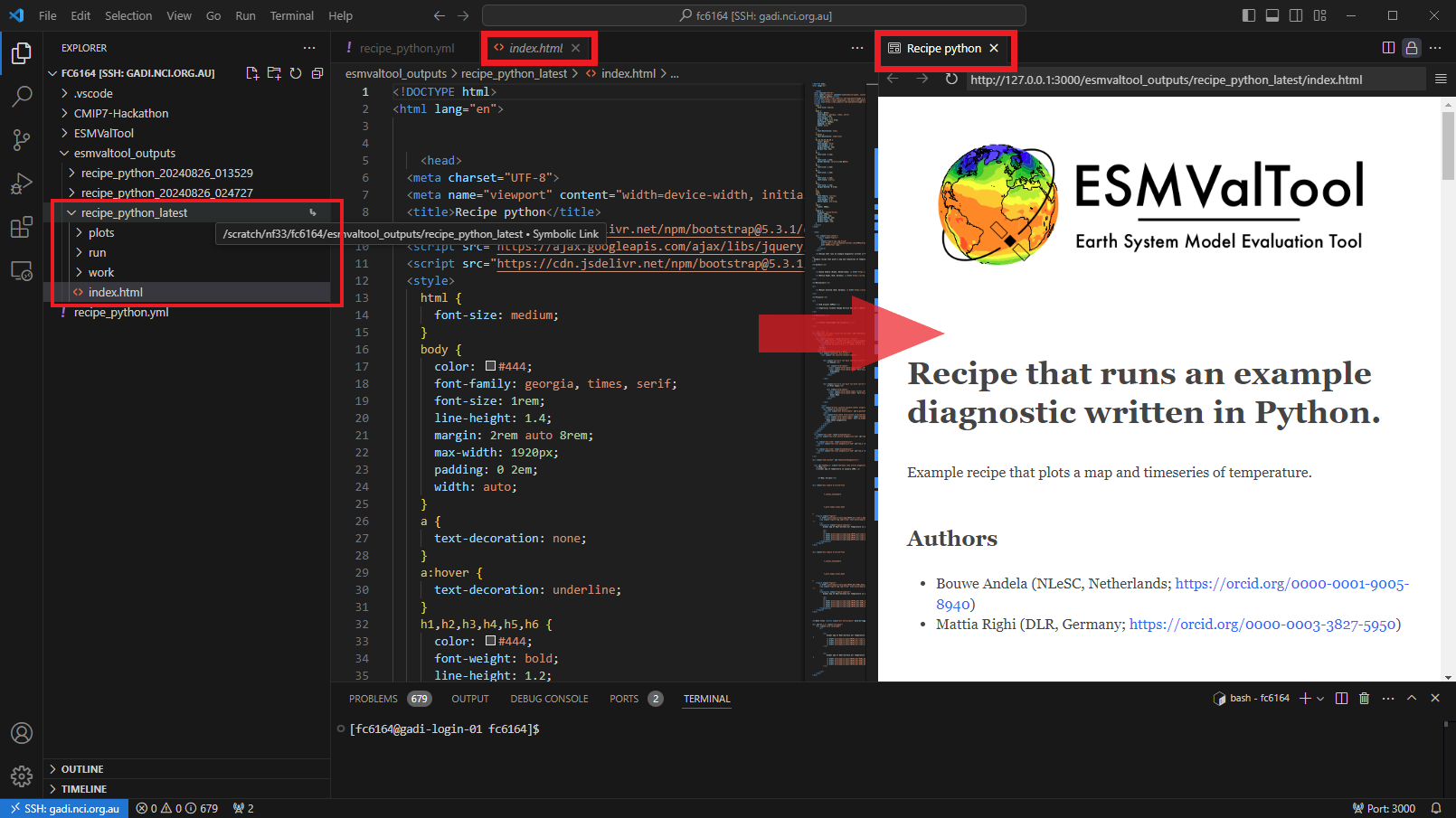
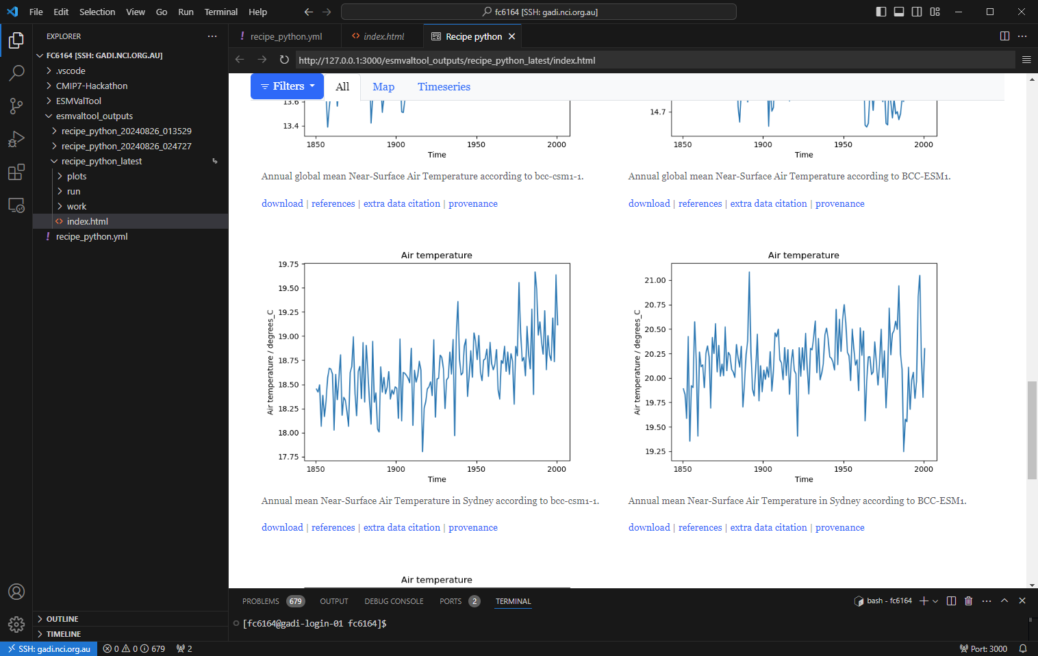
View the output

Now that the recipe runs we can look at the output. We recommend using VS Code with the “Live Preview” extension to view the html that is generated. When you open the html file, you will see the preview button appear in the top right.

Preview

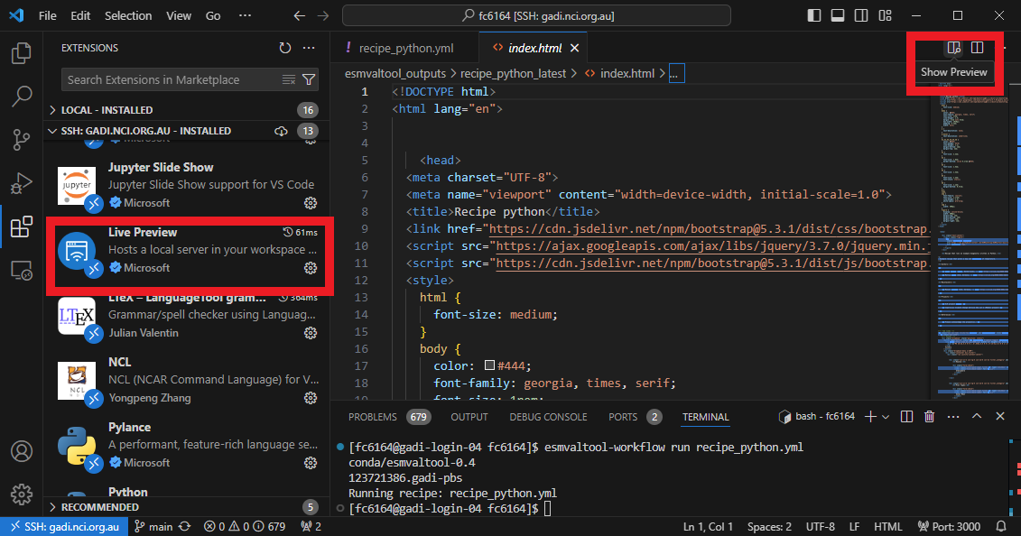
You can see the output folder in explorer with the index.html file with a successful run. When you click on the preview button, the preview will appear to the right. You can also drag this across as a tab to use more of your screen to view.

HTML output

Key Points

• ESMValTool recipes work ‘out of the box’ (if input data is available)

• There are strong links between the recipe, log file, and output folders

• Recipes can easily be modified to re-use existing code for your own use case

Supported data on NCI GADI

Overview

Teaching: 15 min
Exercises: 15 min
Compatibility:

Questions

• What data can I get on Gadi?

• How can I access and find datasets?

Objectives

• Gain knowledge of relevant Gadi projects for data

• How observation data is organised for ESMValTool

• Understanding download and CMORise functions available in ESMValTool

• How observation data is organised for the ILAMB

Introduction

An advantage of using a supercomputer like Gadi at NCI, an ESGF node, is that a lot of data is already available which saves us from searching for and downloading large datasets that can’t be handled on other other computers.

What data can I get on Gadi?

Broadly, the datasets available which can be easily found and read in ESMValTool are:

• Observational data
• ERA5 data
• published CMIP6 data
• published CMIP5 data

What are the NCI projects I need to join?

On NCI, join relevant NCI projects to access that data. The NCI data catalogue can be searched for more information on the collections. Log into NCI with your NCI account to find and join the projects. These would have been checked when you ran the check_hackathon set up.

Data and NCI projects:

• You can check if you’re a member or join ct11 with this link.

The NCI data catalog entries with NCI project:

• ESMValTool observation data collection: ct11
• ESMValTool ERA5 Daily datasets: ct11
• ERA5 : rt52 and ERA5-Land: zz93
• CMIP6 replicas: oi10 and Australian published: fs38 and
• CMIP5 replicas: al33 and Australian: rr3

There is also the NCI project zv30 for CMIP7 collaborative development and evaluation which will be covered later in this episode.

Pro tip: Configuration file rootpaths

Remember the config-user.yml file where we can set directories for ESMValTool to look for the data. This is an example from the Gadi esmvaltool-workflow user configuration:

config rootpaths

rootpath:
  CMIP6: [/g/data/oi10/replicas/CMIP6, /g/data/fs38/publications/CMIP6, /g/data/xp65/public/apps/esmvaltool/replicas/CMIP6]
  CMIP5: [/g/data/r87/DRSv3/CMIP5, /g/data/al33/replicas/CMIP5/combined, /g/data/rr3/publications/CMIP5/output1]
  CMIP3: /g/data/r87/DRSv3/CMIP3
  CORDEX: [/g/data/rr3/publications/CORDEX/output, /g/data/al33/replicas/cordex/output]
  OBS: /g/data/ct11/access-nri/replicas/esmvaltool/obsdata-v2
  OBS6: /g/data/ct11/access-nri/replicas/esmvaltool/obsdata-v2
  obs4MIPs: [/g/data/ct11/access-nri/replicas/esmvaltool/obsdata-v2]
  ana4mips: [/g/data/ct11/access-nri/replicas/esmvaltool/obsdata-v2]
  native6: [/g/data/rt52/era5]
  ACCESS: /g/data/p73/archive/non-CMIP

ESMValTool Tiers

Observational datasets in ESMValTool are organised in tiers reflecting access restriction levels.

• Tier 1 Primarily Obs4MIPS where data is formatted, freely available and ready to use in ESMValTool.
• Tier 2 Data is freely available, CMORised datasets are available in ct11 in ESMValTool.
• Tier 3 These datasets have access rectrictions, licensing and acknowledgement may be required so direct access to the data cannot be provided. ACCESS-NRI can provide support to download and CMORise.

ERA5 in native6 and ERA5 daily in OBS6 Tier3

• native6-era5

The project native6 refers to a collection of datasets that can be read directly into CMIP6 format for use in ESMValTool recipes. ESMValTool supports this with an extra facets file to map the variable names across. This would have been added to your ~/.esmvaltool/extra_facets directory which is also used to fill out default facet values and help find the data. See more information on extra facets.

• ERA5 daily derived

The original hourly data from the “ERA5 hourly data on single levels” and “ERA5 hourly data on pressure levels” collections have been transformed into daily means using the ESMValTool (v2.10) Python package. These are Tier 3 datasets for OBS6. Variables available are: 'clt', 'fx', 'pr', 'prw', 'psl', 'rlds', 'rsds', 'rsdt', 'tas', 'tasmax', 'tasmin', 'tdps', 'ua', 'uas', 'vas'

What is the ESMValTool observation data collection?

We have created a collection of observation datasets that can be pulled directly into ESMValTool. The data has been CMORised, meaning they are netCDF files formatted to CF conventions and CMIP projects. There is a table of available Tier 1 and 2 data which can be found here or you can also expand the below:

Observation collection

long_name	datasets	name
Ambient Aerosol Optical Thickness at 550nm	ESACCI-AEROSOL, MODIS	od550aer
Surface Upwelling Shortwave Radiation	CERES-EBAF, ESACCI-CLOUD, ISCCP-FH	rsus
Carbon Mass Flux out of Atmosphere Due to Net Biospheric Production on Land [kgC m-2 s-1]	GCP2018, GCP2020	nbp
Surface Temperature	CFSR, ESACCI-LST, ESACCI-SST, HadISST, ISCCP-FH, NCEP-NCAR-R1	ts
Daily Maximum Near-Surface Air Temperature	E-OBS, NCEP-NCAR-R1	tasmax
Omega (=dp/dt)	NCEP-NCAR-R1	wap
Surface Dissolved Inorganic Carbon Concentration	OceanSODA-ETHZ	dissicos
Liquid Water Path	ESACCI-CLOUD, MODIS	lwp
Surface Total Alkalinity	OceanSODA-ETHZ	talkos
Eastward Wind	CFSR, NCEP-NCAR-R1	ua
Mole Fraction of N2O	TCOM-N2O	n2o
Grid-Cell Area for Ocean Variables	OceanSODA-ETHZ	areacello
Ambient Aerosol Optical Depth at 870nm	ESACCI-AEROSOL	od870aer
Surface Carbonate Ion Concentration	OceanSODA-ETHZ	co3os
Surface Upwelling Longwave Radiation	CERES-EBAF, ESACCI-CLOUD, ISCCP-FH	rlus
Dissolved Oxygen Concentration	CT2019, ESACCI-GHG, ESRL, GCP2018, GCP2020, Landschuetzer2016, Landschuetzer2020, OceanSODA-ETHZ, Scripps-CO2-KUM, WOA	o2
Specific Humidity	AIRS, AIRS-2-1, HALOE, JRA-25, NCEP-NCAR-R1, NOAA-CIRES-20CR	hus
TOA Outgoing Shortwave Radiation	CERES-EBAF, ESACCI-CLOUD, ISCCP-FH, JRA-25, JRA-55, NCEP-NCAR-R1, NOAA-CIRES-20CR	rsut
Sea Water Salinity	CALIPSO-GOCCP, ESACCI-LANDCOVER, ESACCI-SEA-SURFACE-SALINITY, PHC, WOA	so
Percentage Crop Cover	ESACCI-LANDCOVER	cropFrac
Percentage of the Grid Cell Occupied by Land (Including Lakes)	BerkeleyEarth	sftlf
Sea Surface Temperature	ATSR, HadISST, WOA	tos
Total Dissolved Inorganic Silicon Concentration	CFSR, GLODAP, HadISST, MOBO-DIC_MPIM, OSI-450-nh, OSI-450-sh, OceanSODA-ETHZ, PIOMAS, WOA	si
Daily Minimum Near-Surface Air Temperature	E-OBS, NCEP-NCAR-R1	tasmin
Dissolved Inorganic Carbon Concentration	GLODAP, MOBO-DIC_MPIM, OceanSODA-ETHZ	dissic
Water Vapor Path	ISCCP-FH, JRA-25, NCEP-DOE-R2, NCEP-NCAR-R1, NOAA-CIRES-20CR, SSMI, SSMI-MERIS	prw
Surface Downwelling Longwave Radiation	CERES-EBAF, ISCCP-FH, JRA-55	rlds
Geopotential Height	CFSR, NCEP-NCAR-R1	zg
Northward Wind	CFSR, NCEP-NCAR-R1	va
Relative Humidity	AIRS-2-0, AIRS-2-1, NCEP-DOE-R2, NCEP-NCAR-R1	hur
Tree Cover Percentage	ESACCI-LANDCOVER	treeFrac
Percentage Cover by Shrub	ESACCI-LANDCOVER	shrubFrac
Bare Soil Percentage Area Coverage	ESACCI-LANDCOVER	baresoilFrac
Percentage Cloud Cover	CALIOP, CALIPSO-GOCCP, CloudSat, ESACCI-CLOUD, ISCCP, JRA-25, JRA-55, MODIS, MODIS-1-0, NCEP-DOE-R2, NCEP-NCAR-R1, NOAA-CIRES-20CR, PATMOS-x	cl
Total Alkalinity	GLODAP, OceanSODA-ETHZ	talk
Surface Upwelling Clear-Sky Shortwave Radiation	CERES-EBAF, ESACCI-CLOUD	rsuscs
Mole Fraction of CH4	ESACCI-GHG, TCOM-CH4	ch4
Precipitation	CRU, E-OBS, ESACCI-OZONE, GHCN, GPCC, GPCP-SG, ISCCP-FH, JRA-25, JRA-55, NCEP-DOE-R2, NCEP-NCAR-R1, NOAA-CIRES-20CR, PERSIANN-CDR, REGEN, SSMI, SSMI-MERIS, TRMM-L3, WFDE5, AGCD	pr
Ambient Fine Aerosol Optical Depth at 550nm	ESACCI-AEROSOL	od550lt1aer
Sea Surface Salinity	ESACCI-SEA-SURFACE-SALINITY, WOA	sos
Natural Grass Area Percentage	ESACCI-LANDCOVER	grassFrac
Primary Organic Carbon Production by All Types of Phytoplankton	Eppley-VGPM-MODIS	intpp
Eastward Near-Surface Wind	CFSR	uas
Air Temperature	AIRS, AIRS-2-1, BerkeleyEarth, CFSR, CRU, CowtanWay, E-OBS, GHCN-CAMS, GISTEMP, GLODAP, HadCRUT3, HadCRUT4, HadCRUT5, ISCCP-FH, Kadow2020, NCEP-DOE-R2, NCEP-NCAR-R1, NOAAGlobalTemp, OceanSODA-ETHZ, PHC, WFDE5, WOA	ta
Near-Surface Air Temperature	BerkeleyEarth, CFSR, CRU, CowtanWay, E-OBS, GHCN-CAMS, GISTEMP, HadCRUT3, HadCRUT4, HadCRUT5, ISCCP-FH, Kadow2020, NCEP-NCAR-R1, NOAAGlobalTemp, WFDE5	tas
Surface Downwelling Clear-Sky Longwave Radiation	CERES-EBAF, JRA-55	rldscs
Ambient Aerosol Absorption Optical Thickness at 550nm	ESACCI-AEROSOL	abs550aer
Total Dissolved Inorganic Phosphorus Concentration	WOA	po4
Sea Level Pressure	E-OBS, JRA-55, NCEP-NCAR-R1	psl
Sea Water Potential Temperature	PHC, WOA	thetao
CALIPSO Percentage Cloud Cover	CALIPSO-GOCCP	clcalipso
Surface Aqueous Partial Pressure of CO2	Landschuetzer2016, Landschuetzer2020, OceanSODA-ETHZ	spco2
Mass Concentration of Total Phytoplankton Expressed as Chlorophyll in Sea Water	ESACCI-OC	chl
Surface pH	OceanSODA-ETHZ	phos
TOA Outgoing Clear-Sky Longwave Radiation	CERES-EBAF, ESACCI-CLOUD, ISCCP-FH, JRA-25, JRA-55, NCEP-NCAR-R1	rlutcs
Total Column Ozone	ESACCI-OZONE	toz
Near-Surface Relative Humidity	NCEP-NCAR-R1	hurs
Surface Downward Mass Flux of Carbon as CO2 [kgC m-2 s-1]	GCP2018, GCP2020, Landschuetzer2016, OceanSODA-ETHZ	fgco2
Atmosphere CO2	CT2019, ESRL, Scripps-CO2-KUM	co2s
pH	GLODAP, OceanSODA-ETHZ	ph
Condensed Water Path	MODIS, NOAA-CIRES-20CR	clwvi
Daily-Mean Near-Surface Wind Speed	CFSR, NCEP-NCAR-R1	sfcWind
Surface Downwelling Shortwave Radiation	CERES-EBAF, ISCCP-FH	rsds
TOA Outgoing Clear-Sky Shortwave Radiation	CERES-EBAF, ESACCI-CLOUD, ISCCP-FH, JRA-25, JRA-55, NCEP-NCAR-R1	rsutcs
Total Cloud Cover Percentage	CALIOP, CloudSat, ESACCI-CLOUD, ISCCP, JRA-25, JRA-55, MODIS, MODIS-1-0, NCEP-DOE-R2, NCEP-NCAR-R1, NOAA-CIRES-20CR, PATMOS-x	clt
Convective Cloud Area Percentage	CALIOP, CALIPSO-GOCCP	clc
Northward Near-Surface Wind	CFSR	vas
Surface Air Pressure	CALIPSO-GOCCP, E-OBS, ISCCP-FH, JRA-55, NCEP-NCAR-R1	ps
TOA Outgoing Longwave Radiation	CERES-EBAF, ESACCI-CLOUD, ISCCP-FH, JRA-25, JRA-55, NCEP-NCAR-R1, NOAA-CIRES-20CR	rlut
Delta CO2 Partial Pressure	Landschuetzer2016	dpco2
Surface Downwelling Clear-Sky Shortwave Radiation	CERES-EBAF	rsdscs
TOA Incident Shortwave Radiation	CERES-EBAF, ESACCI-CLOUD, ISCCP-FH	rsdt
Ice Water Path	ESACCI-CLOUD	clivi

ESMValTool data download and CMORise

ESMValTool has the capability to download and format certain observational datasets with data commands, see here for more detail and a table of datasets available to download and format. These are the download and format commands:

esmvaltool data download --config_file <path to config-user.yml>  <dataset-name>
esmvaltool data format --config_file <path to config-user.yml>  <dataset-name>

You will find the ESMValTool facet project for observational data can be OBS or OBS6 where OBS is CMIP5 format and OBS6 is CMIP6 format.

Finding data examples

Find data in recipe

Some facets can have glob patterns or wildcards for values. The facet project cannot be a wildcard, see reference.

An example recipe that will use all CMIP6 datasets and all ensemble members which have a ‘historical’ experiment could look like this:

Solution

datasets:
 - project: CMIP6
   exp: historical
   dataset: '*'
   institute: '*'
   ensemble: '*'
   grid: '*'

Find data using esmvalcore

This can be utilised through the esmvalcore API. To find all available datasets from ESGF which may not be available locally, set search_esgf to always. This example looks for all ensembles for a dataset.

Solution

from esmvalcore import Dataset
from esmvalcore.config import CFG

CFG['search_esgf'] = 'always'
dataset_search = Dataset(
    short_name='tos',
    mip='Omon',
    project='CMIP6',
    exp='historical',
    dataset='ACCESS-ESM1-5',
    ensemble='*',
    grid='gn',
)
ensemble_datasets = list(dataset_search.from_files())
ensemble_datasets

Find all available datasets for a variable in CMIP6

Find all datasets available for variable tos in CMIP6 in concatenated experiments ‘historical’ and ‘ssp585’ for the time range 1850 to 2100.

Solution

template = Dataset(
    short_name='tos',
    mip='Omon',
    activity='CMIP',
    institute='*', # facet req. to search locally
    project='CMIP6',
    exp= ['historical', 'ssp585'],
    dataset='*',  #
    ensemble='*',
    grid='*',
    timerange='1850/2100'  
)

all_datasets = list(template.from_files())
all_datasets

What is ILAMB-Data?

The ILAMB community maintains a collection of reference datasets that have been carefully formatted following CF conventions. ACCESS-NRI hosts a replica of this ILAMB-data collection on NCI-Gadi as part of the ACCESS-NRI Replicated Datasets for Climate Model Evaluation NCI data collection, which can be accessed here. While we ensure this replica is regularly updated, the datasets were initially downloaded from primary sources and reformatted for use within the ILAMB framework. For specific reference information, please check the global attributes within the files.

See something wrong in a dataset? Have a suggestion? This collection is continually evolving and depends on community input. Please submit request for new observation datasets support on the ACCESS-Hive Forum. You can also track progress by following the ILAMB-Data GitHub repository or check out what the ILAMB community users are working on currently on the ILAMB Dataset Integration project board.

Observation collection

Albedo	CERESed4.1, GEWEX.SRB
Biomass	ESACCI, GEOCARBON, NBCD2000, Saatchi2011, Thurner, USForest, XuSaatchi2021
Burned Area	GFED4.1S
Carbon Dioxide	NOAA.Emulated, HIPPOAToM
Diurnal Max Temperature	CRU4.02
Diurnal Min Temperature	CRU4.02
Diurnal Temperature Range	CRU4.02
Ecosystem Respiration	FLUXNET2015, FLUXCOM
Evapotranspiration	GLEAMv3.3a, MODIS, MOD16A2
Global Net Ecosystem Carbon Balance	GCP, Hoffman
Gross Primary Productivity	FLUXNET2015, FLUXCOM, WECANN
Ground Heat Flux	CLASS
Latent Heat	FLUXNET2015, FLUXCOM, DOLCE, CLASS, WECANN
Leaf Area Index	AVHRR, AVH15C1, MODIS
Methane	FluxnetANN
Net Ecosystem Exchange	FLUXNET2015
Nitrogen Fixation	Davies-Barnard
Permafrost	Brown2002, Obu2018
Precipitation	CMAPv1904, FLUXNET2015, GPCCv2018, GPCPv2.3, CLASS
Runoff	Dai, LORA, CLASS
Sensible Heat	FLUXNET2015, FLUXCOM, CLASS, WECANN
Snow Water Equivalent	CanSISE
Soil Carbon	HWSD, NCSCDV22
Surface Air Temperature	CRU4.02, FLUXNET2015
Surface Downward LW Radiation	CERESed4.1, FLUXNET2015, GEWEX.SRB, WRMC.BSRN
Surface Downward SW Radiation	CERESed4.1, FLUXNET2015, GEWEX.SRB, WRMC.BSRN
Surface Net LW Radiation	CERESed4.1, FLUXNET2015, GEWEX.SRB, WRMC.BSRN
Surface Net Radiation	CERESed4.1, FLUXNET2015, GEWEX.SRB, WRMC.BSRN, CLASS
Surface Net SW Radiation	CERESed4.1, FLUXNET2015, GEWEX.SRB, WRMC.BSRN
Surface Relative Humidity	ERA5, CRU4.02
Surface Soil Moisture	WangMao
Surface Upward LW Radiation	CERESed4.1, FLUXNET2015, GEWEX.SRB, WRMC.BSRN
Surface Upward SW Radiation	CERESed4.1, FLUXNET2015, GEWEX.SRB, WRMC.BSRN
Terrestrial Water Storage Anomaly	GRACE

IOMB-DATA list

Alkalinity	GLODAP2.2022
Anthropogenic DIC 1994-2007	Gruber, OCIM
Chlorophyll	GLODAP2.2022, SeaWIFS, MODISAqua
Dissolved Inorganic Carbon	GLODAP2.2022
Nitrate	WOA2018, GLODAP2.2022
Oxygen	WOA2018, GLODAP2.2022
Phosphate	WOA2018, GLODAP2.2022
Salinity	WOA2018, GLODAP2.2022
Silicate	WOA2018, GLODAP2.2022
Temperature	WOA2018, GLODAP2.2022
Vertical Temperature Gradient	WOA2018, GLODAP2.2022

The CMIP7 collaborative development and evaluation project (zv30) on NCI-Gadi

The Australian CMIP7 community, supported by ACCESS-NRI, aims to establish a data space for effectively comparing and evaluating CMIP experiments in preparation for Australia’s forthcoming submission to CMIP7. This shared platform will serve as a collaborative hub, bringing together researchers and model developers to assess model outputs. It will enable comparisons with previous simulations and CMIP6 models, facilitating the real-time exchange of feedback. Additionally, this space will support iterative model improvement by providing a platform for testing and refining model configurations.

This collection is part of the zv30 project on NCI, managed by ACCESS-NRI. Similar to the NCI National data collections, users only have read access to this data. To share a dataset for model evaluation purposes, users must prepare the data according to CF conventions (i.e., CMORize the data) and submit a request to copy the dataset to the zv30 project. To do so, please contact Romain Beucher or Clare Richards at ACCESS-NRI.

If you have not done so already, please join the zv30 project

ZV30 collection in ESMValTool

ESMValTool-workflow on Gadi has been configured to be able to use this collection specifically and differentiate from the rest of the CMIP6 collections.

You can do this by specifying the project facet as ZV30.

In recipe

datasets:
 - project: ZV30
   exp: piControl
   dataset: '*'
   institute: '*'
   ensemble: '*'
   grid: '*'

Key Points

• There is supported data on Gadi to start with using ESMValTool and the ILAMB

Writing your own recipe

Overview

Teaching: 15 min
Exercises: 30 min
Compatibility:

Questions

• How do I create a new recipe?

• Can I use different preprocessors for different variables?

• Can I use different datasets for different variables?

• How can I combine different preprocessor functions?

• Can I run the same recipe for multiple ensemble members?

Objectives

• Create a recipe with multiple preprocessors

• Use different preprocessors for different variables

• Run a recipe with variables from different datasets

Introduction

One of the key strengths of ESMValTool is in making complex analyses reusable and reproducible. But that doesn’t mean everything in ESMValTool needs to be complex. Sometimes, the biggest challenge is in keeping things simple. You probably know the ‘warming stripes’ visualization by Professor Ed Hawkins. On the site https://showyourstripes.info you can find the same visualization for many regions in the world.

Shared by Ed Hawkins under a Creative Commons 4.0 Attribution International licence. Source: https://showyourstripes.info

In this episode, we will reproduce and extend this functionality with ESMValTool. We have prepared a small Python script that takes a NetCDF file with timeseries data, and visualizes it in the form of our desired warming stripes figure.

As part of your setup when you ran check_hackathon you will have a clone of this repo in your scratch training space.

The diagnostic script that we will use is called warming_stripes.py and can be found in your cloned Hackathon folder: /scratch/nf33/$USER/CMIP7-Hackathon/exercises/WritingYourOwnRecipe.

You may also have a look at the contents, but it is not necessary to do so for this lesson.

We will write an ESMValTool recipe that takes some data, performs the necessary preprocessing, and then runs this Python script.

Drawing up a plan

Previously, we saw that running ESMValTool executes a number of tasks. What tasks do you think we will need to execute and what should each of these tasks do to generate the warming stripes?

Answer

In this episode, we will need to do the following two tasks:

• A preprocessing task that converts the gridded temperature data to a timeseries of global temperature anomalies
• A diagnostic task that calls our Python script, taking our preprocessed timeseries data as input.

Building a recipe from scratch

The easiest way to make a new recipe is to start from an existing one, and modify it until it does exactly what you need. However, in this episode we will start from scratch. This forces us to think about all the steps involved in processing the data. We will also deal with commonly occurring errors through the development of the recipe.

Remember the basic structure of a recipe, and notice that each component is extensively described in the documentation under the section, “Overview”:

• documentation
• datasets
• preprocessors
• diagnostics

This is the first place to look for help if you get stuck.

Create file and run on Gadi

Open VS Code with a remote SSH connection to Gadi with your /scratch/nf33/$USER folder in your workspace. Refer to VS Code setup Create a new file called recipe_warming_stripes.yml in your working directory for this exercise. Let’s add the standard header comments (these do not do anything), and a first description.

# ESMValTool
# recipe_warming_stripes.yml
---
documentation:
  description: Reproducing Ed Hawkins' warming stripes visualization
  title: Reproducing Ed Hawkins' warming stripes visualization.

Notice that yaml always requires two spaces indentation between the different levels. Save the file in VS Code with ctrl + s.

Reminder: how to run recipe

In the terminal, load the module to use ESMValTool on Gadi. If you don’t have a terminal open, the shortcut in VS Code is Ctrl + `. Add the full path (eg. /scratch/nf33/$USER) to your recipe_warming_stripes.yml in this when you run your recipe or cd to the directory. Also ensure that you are on the project nf33.

switchproj nf33
module use /g/data/xp65/public/modules
module load esmvaltool-workflow

esmvaltool-workflow run --output_dir=/scratch/nf33/$USER/esmvaltool_outputs <dir_path>/recipe_warming_stripes.yml

If you try to run this, it would give an error. Below you see the last few lines of the error message.

...
yamale.yamale_error.YamaleError: 
Error validating data '/home/users/username/esmvaltool_tutorial/recipe_warming_stripes.yml' 
with schema 
'/apps/jasmin/community/esmvaltool/miniconda3_py311_23.11.0-2/envs/esmvaltool/lib/python3.11/
site-packages/esmvalcore/_recipe/recipe_schema.yml'
	documentation.authors: Required field missing
2024-05-27 13:21:23,805 UTC [41924] INFO    
If you have a question or need help, please start a new discussion on 
https://github.com/ESMValGroup/ESMValTool/discussions
If you suspect this is a bug, please open an issue on 
https://github.com/ESMValGroup/ESMValTool/issues
To make it easier to find out what the problem is, please consider attaching the 
files run/recipe_*.yml and run/main_log_debug.txt from the output directory.

We can use the log message above, to understand why ESMValTool failed. Here, this is because we missed a required field with author names. The text documentation.authors: Required field missing tells us that. We see that ESMValTool always tries to validate the recipe at an early stage. Note also the suggestion to open a GitHub issue if you need help debugging the error message. This is something most users do when they cannot understand the error or are not able to fix it on their own.

Let’s add some additional information to the recipe. Open the recipe file again, and add an authors section below the description. ESMValTool expects the authors as a list, like so:

authors:
  - lastname_firstname

To bypass a number of similar error messages, add a minimal diagnostics section below the documentation. The file should now look like:

# ESMValTool
# recipe_warming_stripes.yml
---
documentation:
  description: Reproducing Ed Hawkins' warming stripes visualization
  title: Reproducing Ed Hawkins' warming stripes visualization.

  authors:
    - doe_john
diagnostics:
  dummy_diagnostic_1:
    scripts: null

This is the minimal recipe layout that is required by ESMValTool. If we now run the recipe again, you will probably see the following error:

ValueError: Tag 'doe_john' does not exist in section 
'authors' of /apps/jasmin/community/esmvaltool/ESMValTool_2.10.0/esmvaltool/config-references.yml

Pro tip: config-references.yml

The error message above points to a file named config-references.yml This is where ESMValTool stores all its citation information. To add yourself as an author, you will need to use and run ESMValTool in developer mode, then add your name in the form lastname_firstname in alphabetical order following the existing entries, under the # Development team section. The file used in this Gadi module doesn’t have editing permissions so use an existing author. See the List of authors section in the ESMValTool documentation for more information.

For now, let’s just use one of the existing references. Change the author field to righi_mattia, who cannot receive enough credit for all the effort he put into ESMValTool. If you now run the recipe, you would see the final message

ERROR   No tasks to run!

Although there is no actual error in the recipe, ESMValTool assumes you mistakenly left out a variable name to process and alerts you with this error message.

Adding a dataset entry

Let’s add a datasets section.

Filling in the dataset keys

Use the paths specified in the configuration file to explore the data directory, and look at the explanation of the dataset entry in the ESMValTool documentation. For two datasets, write down the following properties:

• project
• variable (short name)
• CMIP table
• dataset (model name or obs/reanalysis dataset)
• experiment
• ensemble member
• grid
• start year
• end year

Answers

Here we have chosen a CMIP6 and CMIP5 ACCESS dataset.

key	file 1	file 2
project	CMIP6	CMIP5
short name	tas	tas
CMIP table	Amon	Amon
dataset	ACCESS-ESM1-5	ACCESS1-0
experiment	historical	historical
ensemble	r1i1p1f1	r1i1p1
grid	gn (native grid)	N/A
start year	1850	1850
end year	2014	2005

Note that the grid key is only required for CMIP6 data, and that the extent of the historical period has changed between CMIP5 and CMIP6.

Let us start with the ACCESS-ESM1-5 dataset and add a ‘datasets’ section to the recipe, listing this single dataset, as shown below. Note that key fields such as mip or start_year are included in the datasets section here but are part of the diagnostic section in the recipe example seen in Running your first recipe.

# ESMValTool
# recipe_warming_stripes.yml
---
documentation:
  description: Reproducing Ed Hawkins' warming stripes visualization
  title: Reproducing Ed Hawkins' warming stripes visualization.

  authors:
    - righi_mattia
datasets:
  - {dataset: ACCESS-ESM1-5, project: CMIP6, mip: Amon, exp: historical, 
     ensemble: r1i1p1f1, grid: gn, start_year: 1850, end_year: 2014}

diagnostics:
  dummy_diagnostic_1:
    scripts: null

The recipe should run but produce the same message as in the previous case since we still have not included a variable to actually process. We have not included the short name of the variable in this dataset section because this allows us to reuse this dataset entry with different variable names later on. This is not really necessary for our simple use case, but it is common practice in ESMValTool.

Pro-tip: Automatically populating a recipe with all available datasets

You can select all available models for processing using glob patterns or wildcards. Seen in Supported data on Gadi exercises on finding data.

Adding the preprocessor section

Above, we already described the preprocessing task that needs to convert the standard, gridded temperature data to a timeseries of temperature anomalies.

Defining the preprocessor

Have a look at the available preprocessors in the documentation. Write down

• Which preprocessor functions do you think we should use?
• What are the parameters that we can pass to these functions?
• What do you think should be the order of the preprocessors?
• A suitable name for the overall preprocessor

Solution

We need to calculate anomalies and global means. There is an anomalies preprocessor which takes in as arguments, a time period, a reference period, and whether or not to standardize the data. The global means can be calculated with the area_statistics preprocessor, which takes an operator as argument (in our case we want to compute the mean).

The default order in which these preprocessors are applied can be seen here: area_statistics comes before anomalies. If you want to change this, you can use the custom_order preprocessor as described here. For this example, we will keep the default order.

Let’s name our preprocessor global_anomalies.

Add the following block to your recipe file between the datasets and diagnostics block:

preprocessors:
  global_anomalies:
    area_statistics:
      operator: mean
    anomalies:
        period: month
        reference:
          start_year: 1981
          start_month: 1
          start_day: 1
          end_year: 2010
          end_month: 12
          end_day: 31
        standardize: false

Completing the diagnostics section

We are now ready to finish our diagnostics section. Remember that we want to create two tasks: a preprocessor task, and a diagnostic task. To illustrate that we can also pass settings to the diagnostic script, we add the option to specify a custom colormap.

Fill in the blanks

Extend the diagnostics section in your recipe by filling in the blanks in the following template:

diagnostics:
  <... (suitable name for our diagnostic)>:
    description: <...>
    variables:
      <... (suitable name for the preprocessed variable)>:
        short_name: <...>
        preprocessor: <...>
    scripts:
      <... (suitable name for our python script)>:
        script: <full path to python script>
        colormap: <... choose from matplotlib colormaps>

Solution

diagnostics:
  diagnostic_warming_stripes:
    description: visualize global temperature anomalies as warming stripes
    variables:
      global_temperature_anomalies:
        short_name: tas
        preprocessor: global_anomalies
    scripts:
      warming_stripes_script:
        script: /scratch/nf33/$USER/CMIP7-Hackathon/exercises/WritingYourOwnRecipe/warming_stripes.py
        colormap: 'bwr'

You should now be able to run the recipe from your working directory to get your own warming stripes.

esmvaltool-workflow run recipe_warming_stripes.yml

Find the plots in the plot directory of the output run eg.

/scratch/nf33/fc6164/esmvaltool_outputs/recipe_warming_latest/plots
└── diagnostic_warming_stripes
    └── warming_stripes_script
        └── CMIP6_ACCESS-ESM1-5_Amon_historical_r1i1p1f1_global_temperature_anomalies_gn_1850-2014.png

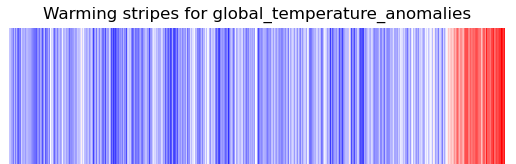
Note

For the purpose of simplicity in this episode, we have not added logging or provenance tracking in the diagnostic script. Once you start to develop your own diagnostic scripts and want to add them to the ESMValTool repositories, this will be required. Writing your own diagnostic script is discussed in a later episode.

Bonus exercises

Below are a few exercises to practice modifying an ESMValTool recipe. For your reference, a copy of the recipe at this point can be found in the solution_recipes folder: /scratch/nf33/$USER/CMIP7-Hackathon/exercises/Exercise2_files/solution_recipes. Note the full path to the script will differ.
This will be the point of departure for each of the modifications we’ll make below. An example of the modified recipes are also in this folder

Specific location selection

On showyourstripes.org, you can download stripes for specific locations. Here we show how this can be done with ESMValTool. Instead of the global mean, we can pick a location to plot the stripes for. Can you find a suitable preprocessor to do this?

Solution

You can use extract_point or extract_region to select a location. We used extract_region for Australia. A copy is called recipe_warming_stripes_local.yml and this is the difference from the previous recipe:

--- recipe_warming_stripes.yml
+++ recipe_warming_stripes_local.yml
@@ -10,9 +10,11 @@
   - {dataset: ACCESS-ESM1-5, project: CMIP6, mip: Amon, exp: historical, 
      ensemble: r1i1p1f1, grid: gn, start_year: 1850, end_year: 2014}

 preprocessors:
-  global_anomalies:
+  aus_anomalies:
+    extract_region:
+      start_longitude: 110
+      end_longitude: 160
+      start_latitude: -45
+      end_latitude: -9
     area_statistics:
       operator: mean
     anomalies:
       period: month
       reference:
@@ -29,9 +32,9 @@
 diagnostics:
   diagnostic_warming_stripes:
     variables:
-      global_temperature_anomalies:
+      temperature_anomalies_aus:
         short_name: tas
-        preprocessor: global_anomalies
+        preprocessor: aus_anomalies
     scripts:
       warming_stripes_script:
         script: /scratch/nf33/$USER/CMIP7-Hackathon/exercises/WritingYourOwnRecipe/warming_stripes.py

Different time periods

Split the diagnostic in two with two different time periods for the same variable. You can choose the time periods yourself. In the example below, we have chosen the recent past and the 20th century and have used variable grouping.

Solution

This is the difference with the previous recipe:

--- recipe_warming_stripes_local.yml
+++ recipe_warming_stripes_periods.yml
@@ -7,7 +7,7 @@

 datasets:
-  - {dataset: ACCESS-ESM1-5, project: CMIP6, mip: Amon, exp: historical, 
-  	  ensemble: r1i1p1f1, grid: gn, start_year: 1850, end_year: 2014}
+  - {dataset: ACCESS-ESM1-5, project: CMIP6, mip: Amon, exp: historical, 
+     ensemble: r1i1p1f1, grid: gn}

 preprocessors:
   anomalies_aus:
@@ -31,9 +31,16 @@
diagnostics:
  diagnostic_warming_stripes:
    variables:
-      temperature_anomalies_aus:
+      temperature_anomalies_recent:
         short_name: tas
         preprocessor: anomalies_aus
+        start_year: 1950
+        end_year: 2014
+      temperature_anomalies_20th_century:
+        short_name: tas
+        preprocessor: anomalies_aus
+        start_year: 1900
+        end_year: 1999
     scripts:
       warming_stripes_script:
         script: /scratch/nf33/$USER/CMIP7-Hackathon/exercises/WritingYourOwnRecipe/warming_stripes.py

Different preprocessors

Now that you have different variable groups, we can also use different preprocessors. Add a second preprocessor to add another location of your choosing.

Solution

This is the difference with the previous recipe:

--- recipe_warming_stripes_periods.yml
+++ recipe_warming_stripes_multiple_locations.yml
@@ -19,7 +19,7 @@
       end_latitude: -9
     area_statistics:
       operator: mean
-    anomalies:
+    anomalies: &anomalies
       period: month
       reference:
         start_year: 1981
@@ -29,18 +29,24 @@
         end_month: 12
         end_day: 31
       standardize: false
+  anomalies_sydney:
+    extract_point:
+      latitude: -34
+      longitude: 151
+      scheme: linear
+    anomalies: *anomalies

 diagnostics:
   diagnostic_warming_stripes:
     variables:
-      temperature_anomalies_recent:
+      temperature_anomalies_recent_aus:
         short_name: tas
         preprocessor: anomalies_amsterdam
         start_year: 1950
         end_year: 2014
-      temperature_anomalies_20th_century:
+      temperature_anomalies_20th_century_sydney:
         short_name: tas
-        preprocessor: anomalies_amsterdam
+        preprocessor: anomalies_sydney
         start_year: 1900
         end_year: 1999
     scripts:

Pro-tip: YAML anchors

If you want to avoid retyping the arguments used in your preprocessor, you can use YAML anchors as seen in the anomalies preprocessor specifications in the recipe above.

Additional datasets

So far we have defined the datasets in the datasets section of the recipe. However, it’s also possible to add specific datasets only for specific variables or variable groups. Take a look at the documentation to learn about the additional_datasets keyword here, and add a second dataset only for one of the variable groups.

Solution

This is the difference with the previous recipe:

--- recipe_warming_stripes_multiple_locations.yml
+++ recipe_warming_stripes_additional_datasets.yml
@@ -49,6 +49,8 @@
         preprocessor: anomalies_sydney
         start_year: 1900
         end_year: 1999
+        additional_datasets:
+          - {dataset: ACCESS1-3, project: CMIP5, mip: Amon, exp: historical, ensemble: r1i1p1}
     scripts:
       warming_stripes_script:
         script: /scratch/nf33/$USER/CMIP7-Hackathon/exercises/WritingYourOwnRecipe/warming_stripes.py

Multiple ensemble members

You can choose data from multiple ensemble members for a model in a single line.

Solution

The dataset section allows you to choose more than one ensemble member Changes made are shown in the diff output below:

--- recipe_warming_stripes.yml	
+++ recipe_warming_stripes_multiple_ensemble_members.yml	
@@ -10,7 +10,7 @@
-     ensemble: r1i1p1f1, grid: gn, start_year: 1850, end_year: 2014}
+     ensemble: "r(1:2)i1p1f1", grid: gn, start_year: 1850, end_year: 2014}

Pro-tip: Concatenating datasets

Check out the section on a different way to use multiple ensemble members or even multiple experiments at Concatenating data corresponding to multiple facets.

Key Points

• A recipe can work with different preprocessors at the same time.

• The setting additional_datasets can be used to add a different dataset.

• Variable groups are useful for defining different settings for different variables.

• Multiple ensemble members and experiments can be analysed in a single recipe through concatenation.

Writing your own diagnostic script

Overview

Teaching: 20 min
Exercises: 30 min
Compatibility:

Questions

• How do I write a new diagnostic in ESMValTool?

• How do I use the preprocessor output in a Python diagnostic?

Objectives

• Write a new Python diagnostic script.

• Explain how a diagnostic script reads the preprocessor output.

Introduction

The diagnostic script is an important component of ESMValTool and it is where the scientific analysis or performance metric is implemented. With ESMValTool, you can adapt an existing diagnostic or write a new script from scratch. Diagnostics can be written in a number of open source languages such as Python, R, Julia and NCL but we will focus on understanding and writing Python diagnostics in this lesson.

In this lesson, we will explain how to find an existing diagnostic and run it. Also, we will work with the recipe recipe_python.yml and the diagnostic script diagnostic.py called by this recipe that we have seen in the lesson Running your first recipe.

Let’s get started!

Understanding an existing Python diagnostic

A clone of the ESMValTool repository should be available in your user folder in the nf33 scratch folder (/scratch/nf33/$USER/ESMValTool). If not, please make sure to run the check_hackathon command after loading the esmvaltool-workflow module, check for any errors.

The folder ESMValTool contains the source code of the tool. We can find the recipe recipe_python.yml and the python script diagnostic.py in these directories:

• ESMValTool/esmvaltool/recipes/examples/recipe_python.yml
• ESMValTool/esmvaltool/diag_scripts/examples/diagnostic.py

Let’s have look at the code in diagnostic.py. For reference, we show the diagnostic code in the dropdown box below. There are four main sections in the script:

• A description i.e. the docstring (line 1).
• Import statements (line 2-16).
• Functions that implement our analysis (line 21-102).
• A typical Python top-level script i.e. if __name__ == '__main__' (line 105-108).

diagnostic.py

 1:  """Python example diagnostic."""
 2:  import logging
 3:  from pathlib import Path
 4:  from pprint import pformat
 5:
 6:  import iris
 7:
 8:  from esmvaltool.diag_scripts.shared import (
 9:      group_metadata,
10:      run_diagnostic,
11:      save_data,
12:      save_figure,
13:      select_metadata,
14:      sorted_metadata,
15:  )
16:  from esmvaltool.diag_scripts.shared.plot import quickplot
17:
18:  logger = logging.getLogger(Path(__file__).stem)
19:
20:
21:  def get_provenance_record(attributes, ancestor_files):
22:      """Create a provenance record describing the diagnostic data and plot."""
23:      caption = caption = attributes['caption'].format(**attributes)
24:
25:      record = {
26:          'caption': caption,
27:          'statistics': ['mean'],
28:          'domains': ['global'],
29:          'plot_types': ['zonal'],
30:          'authors': [
31:              'andela_bouwe',
32:              'righi_mattia',
33:          ],
34:          'references': [
35:              'acknow_project',
36:          ],
37:          'ancestors': ancestor_files,
38:      }
39:      return record
40:
41:
42:  def compute_diagnostic(filename):
43:      """Compute an example diagnostic."""
44:      logger.debug("Loading %s", filename)
45:      cube = iris.load_cube(filename)
46:
47:      logger.debug("Running example computation")
48:      cube = iris.util.squeeze(cube)
49:      return cube
50:
51:
52:  def plot_diagnostic(cube, basename, provenance_record, cfg):
53:      """Create diagnostic data and plot it."""
54:
55:      # Save the data used for the plot
56:      save_data(basename, provenance_record, cfg, cube)
57:
58:      if cfg.get('quickplot'):
59:          # Create the plot
60:          quickplot(cube, **cfg['quickplot'])
61:          # And save the plot
62:          save_figure(basename, provenance_record, cfg)
63:
64:
65:  def main(cfg):
66:      """Compute the time average for each input dataset."""
67:      # Get a description of the preprocessed data that we will use as input.
68:      input_data = cfg['input_data'].values()
69:
70:      # Demonstrate use of metadata access convenience functions.
71:      selection = select_metadata(input_data, short_name='tas', project='CMIP5')
72:      logger.info("Example of how to select only CMIP5 temperature data:\n%s",
73:                  pformat(selection))
74:
75:      selection = sorted_metadata(selection, sort='dataset')
76:      logger.info("Example of how to sort this selection by dataset:\n%s",
77:                  pformat(selection))
78:
79:      grouped_input_data = group_metadata(input_data,
80:                                          'variable_group',
81:                                          sort='dataset')
82:      logger.info(
83:          "Example of how to group and sort input data by variable groups from "
84:          "the recipe:\n%s", pformat(grouped_input_data))
85:
86:      # Example of how to loop over variables/datasets in alphabetical order
87:      groups = group_metadata(input_data, 'variable_group', sort='dataset')
88:      for group_name in groups:
89:          logger.info("Processing variable %s", group_name)
90:          for attributes in groups[group_name]:
91:              logger.info("Processing dataset %s", attributes['dataset'])
92:              input_file = attributes['filename']
93:              cube = compute_diagnostic(input_file)
94:
95:              output_basename = Path(input_file).stem
96:              if group_name != attributes['short_name']:
97:                  output_basename = group_name + '_' + output_basename
98:              if "caption" not in attributes:
99:                  attributes['caption'] = input_file
100:              provenance_record = get_provenance_record(
101:                  attributes, ancestor_files=[input_file])
102:              plot_diagnostic(cube, output_basename, provenance_record, cfg)
103:
104:
105:  if __name__ == '__main__':
106:
107:      with run_diagnostic() as config:
108:          main(config)

What is the starting point of a diagnostic?

1. Can you spot a function called main in the code above?
2. What are its input arguments?
3. How many times is this function mentioned?

Solution

1. The main function is defined in line 65 as main(cfg).
2. The input argument to this function is the variable cfg, a Python dictionary that holds all the necessary information needed to run the diagnostic script such as the location of input data and various settings. We will next parse this cfg variable in the main function and extract information as needed to do our analyses (e.g. in line 68).
3. The main function is called near the very end on line 108. So, it is mentioned twice in our code - once where it is called by the top-level Python script and second where it is defined.

The function run_diagnostic

The function run_diagnostic (line 107) is called a context manager provided with ESMValTool and is the main entry point for most Python diagnostics.

Create a copy of the files for you to edit

You would already have a copy of the recipe_python.yml from the lesson Running your first recipe. Use the file you edited after you ran

esmvaltool recipes get examples/recipe_python.yml

Use the edited file from the completion of the lesson.

Copy the file diagnostic.py to your working folder to keep the ones in the repo as templates unaltered while you can more easily find the files you are editing. Edit your recipe to point to your copy of diagnostic.py. Also, note the location for when you run your recipe.

Solution

Example of your working folder:

/scratch/nf33/$USER/Exercise_writeDiagnostic/recipe_python.yml
/scratch/nf33/$USER/Exercise_writeDiagnostic/diagnostic.py

In your recipe_python.yml, edit the path to the diagnostic script.

    script1:
      script: /scratch/nf33/$USER/Exercise_writeDiagnostic/diagnostic.py
      quickplot:

When running the recipe you can run to the full path of your recipe if you are not in that directory:

esmvaltool-workflow run /scratch/nf33/$USER/Exercise_writeDiagnostic/recipe_python.yml

Preprocessor-diagnostic interface

In the previous exercise, we have seen that the variable cfg is the input argument of the main function. The first argument passed to the diagnostic via the cfg dictionary is a path to a file called settings.yml. The ESMValTool documentation page provides an overview of what is in this file, see Diagnostic script interfaces.

What information do I need when writing a diagnostic script?

Load the module in Gadi if you haven’t already. We know how to change the configuration settings before running a recipe. First we set the option remove_preproc_dir to false in the configuration file, then run the recipe recipe_python.yml: (Or look at the output folder from your previous working run.)

module use /g/data/xp65/public/modules
module load esmvaltool-workflow

esmvaltool-workflow run <your_working_folder>/recipe_python.yml

1. Can you find one example of the file settings.yml in the run directory?
2. Open the file settings.yml and look at the input_files list. It contains paths to some files metadata.yml. What information do you think is saved in those files?

Solution

1. One example of settings.yml can be found in the directory: /scratch/nf33/[username]/esmvaltool_outputs/recipe_python_latest/run/map/script1/settings.yml
2. The metadata.yml files hold information about the preprocessed data. There is one file for each variable having detailed information on your data including project (e.g., CMIP6, CMIP5), dataset names (e.g., BCC-ESM1, CanESM2), variable attributes (e.g., standard_name, units), preprocessor applied and time range of the data. You can use all of this information in your own diagnostic.

Diagnostic shared functions

Looking at the code in diagnostic.py, we see that input_data is read from the cfg dictionary (line 68). Now we can group the input_data according to some criteria such as the model or experiment. To do so, ESMValTool provides many functions such as select_metadata (line 71), sorted_metadata (line 75), and group_metadata (line 79). As you can see in line 8, these functions are imported from esmvaltool.diag_scripts.shared that means these are shared across several diagnostics scripts. A list of available functions and their description can be found in The ESMValTool Diagnostic API reference.

Extracting information needed for analysis

We have seen the functions used for selecting, sorting and grouping data in the script. What do these functions do?

Solution

There is a statement after use of select_metadata, sorted_metadata and group_metadata that starts with logger.info (lines 72, 76 and 82). These lines print output to the log files. In the previous exercise, we ran the recipe recipe_python.yml. If you look at the log file recipe_python_#_#/run/map/script1/log.txt in esmvaltool_output directory, you can see the output from each of these functions, for example:

2023-06-28 12:47:14,038 [2548510] INFO     diagnostic,106	Example of how to
group and sort input data by variable groups from the recipe:
{'tas': [{'alias': 'CMIP5',
         'caption': 'Global map of {long_name} in January 2000 according to '
                    '{dataset}.\n',
         'dataset': 'bcc-csm1-1',
         'diagnostic': 'map',
         'end_year': 2000,
         'ensemble': 'r1i1p1',
         'exp': 'historical',
         'filename': '~/recipe_python_20230628_124639/preproc/map/tas/
               CMIP5_bcc-csm1-1_Amon_historical_r1i1p1_tas_2000-P1M.nc',
         'frequency': 'mon',
         'institute': ['BCC'],
         'long_name': 'Near-Surface Air Temperature',
         'mip': 'Amon',
         'modeling_realm': ['atmos'],
         'preprocessor': 'to_degrees_c',
         'product': ['output1', 'output2'],
         'project': 'CMIP5',
         'recipe_dataset_index': 1,
         'short_name': 'tas',
         'standard_name': 'air_temperature',
         'start_year': 2000,
         'timerange': '2000/P1M',
         'units': 'degrees_C',
         'variable_group': 'tas',
         'version': 'v1'},
        {'activity': 'CMIP',
         'alias': 'CMIP6',
         'caption': 'Global map of {long_name} in January 2000 according to '
                    '{dataset}.\n',
         'dataset': 'BCC-ESM1',
         'diagnostic': 'map',
         'end_year': 2000,
         'ensemble': 'r1i1p1f1',
         'exp': 'historical',
         'filename': '~/recipe_python_20230628_124639/preproc/map/tas/
               CMIP6_BCC-ESM1_Amon_historical_r1i1p1f1_tas_gn_2000-P1M.nc',
         'frequency': 'mon',
         'grid': 'gn',
         'institute': ['BCC'],
         'long_name': 'Near-Surface Air Temperature',
         'mip': 'Amon',
         'modeling_realm': ['atmos'],
         'preprocessor': 'to_degrees_c',
         'project': 'CMIP6',
         'recipe_dataset_index': 0,
         'short_name': 'tas',
         'standard_name': 'air_temperature',
         'start_year': 2000,
         'timerange': '2000/P1M',
         'units': 'degrees_C',
         'variable_group': 'tas',
         'version': 'v20181214'}]}

This is how we can access preprocessed data within our diagnostic.

Diagnostic computation

After grouping and selecting data, we can read individual attributes (such as filename) of each item. Here, we have grouped the input data by variables, so we loop over the variables (line 88). Following this is a call to the function compute_diagnostic (line 93). Let’s look at the definition of this function in line 42, where the actual analysis of the data is done.

Note that output from the ESMValCore preprocessor is in the form of NetCDF files. Here, compute_diagnostic uses Iris to read data from a netCDF file and performs an operation squeeze to remove any dimensions of length one. We can adapt this function to add our own analysis. As an example, here we calculate the bias using the average of the data using Iris cubes.

def compute_diagnostic(filename):
    """Compute an example diagnostic."""
    logger.debug("Loading %s", filename)
    cube = iris.load_cube(filename)

    logger.debug("Running example computation")
    cube = iris.util.squeeze(cube)

    # Calculate a bias using the average of data
    cube.data = cube.core_data() - cube.core_data.mean()
    return cube

iris cubes

Iris reads data from NetCDF files into data structures called cubes. The data in these cubes can be modified, combined with other cubes’ data or plotted.

Reading data using xarray

Alternately, you can use xarray to read the data instead of Iris.

Solution

First, import xarray package at the top of the script as:

import xarray as xr

Then, change the compute_diagnostic as:

def compute_diagnostic(filename):
   """Compute an example diagnostic."""
   logger.debug("Loading %s", filename)
   dataset = xr.open_dataset(filename)

   #do your analyses on the data here

   return dataset

Caution: If you read data using xarray keep in mind to change accordingly the other functions in the diagnostic which are dealing at the moment with Iris cubes.

Reading data using the netCDF4 package

Yet another option to read the NetCDF file data is to use the netCDF-4 Python interface to the netCDF C library.

Solution

First, import the netCDF4 package at the top of the script as:

import netCDF4

Then, change compute_diagnostic as:

def compute_diagnostic(filename):
   """Compute an example diagnostic."""
   logger.debug("Loading %s", filename)
   nc_data = netCDF4.Dataset(filename,'r')

   #do your analyses on the data here

   return nc_data

Caution: If you read data using netCDF4 keep in mind to change accordingly the other functions in the diagnostic which are dealing at the moment with Iris cubes.

Diagnostic output

Plotting the output

Often, the end product of a diagnostic script is a plot or figure. The Iris cube returned from the compute_diagnostic function (line 93) is passed to the plot_diagnostic function (line 102). Let’s have a look at the definition of this function in line 52. This is where we would plug in our plotting routine in the diagnostic script.

More specifically, the quickplot function (line 60) can be replaced with the function of our choice. As can be seen, this function uses **cfg['quickplot'] as an input argument. If you look at the diagnostic section in the recipe recipe_python.yml, you see quickplot is a key there:

    script1:
      script: <path_to_script diagnostic.py>
      quickplot:
        plot_type: pcolormesh
        cmap: Reds

This way, we can pass arguments such as the type of plot pcolormesh and the colormap cmap:Reds from the recipe to the quickplot function in the diagnostic.

Passing arguments from the recipe to the diagnostic

Change the type of the plot and its colormap and inspect the output figure.

Solution

In the recipe recipe_python.yml, you could change plot_type and cmap. As an example, we choose plot_type: pcolor and cmap: BuGn:

    script1:
      script: <path_to_script diagnostic.py>
      quickplot:
        plot_type: pcolor
        cmap: BuGn

The plot can be found at path_to_recipe_output/plots/map/script1/png.

ESMValTool gallery

ESMValTool makes it possible to produce a wide array of plots and figures as seen in the gallery.

Saving the output

In our example, the function save_data in line 56 is used to save the Iris cube. The saved files can be found under the work directory in a .nc format. There is also the function save_figure in line 62 to save the plots under the plot directory in a .png format (or preferred format specified in your configuration settings). Again, you may choose your own method of saving the output.

## in diagnostic.py ##
55:      # Save the data used for the plot
56:      save_data(basename, provenance_record, cfg, cube)
..
61:          # And save the plot
62:          save_figure(basename, provenance_record, cfg)

You will see that they are imported from esmvaltool.diag_scripts.shared and take arguments such as cfg so that they can be saved in the appropriate output location.

Recording the provenance

When developing a diagnostic script, it is good practice to record provenance. To do so, we use the function get_provenance_record (line 100). Let us have a look at the definition of this function in line 21 where we describe the diagnostic data and plot. Using the dictionary record, it is possible to add custom provenance to our diagnostics output. Provenance is stored in the W3C PROV XML format and also in an SVG file under the work and plot directory. For more information, see recording provenance. You will see that the record gets parsed as an argument in the saving outputs functions above.

Congratulations!

You now know the basic diagnostic script structure and some available tools for putting together your own diagnostics. Have a look at existing recipes and diagnostics in the repository for more examples of functions you can use in your diagnostics!

Key Points

• ESMValTool provides helper functions to interface a Python diagnostic script with preprocessor output.

• Existing diagnostics can be used as templates and modified to write new diagnostics.

• Helper functions can be imported from esmvaltool.diag_scripts.shared and used in your own diagnostic script.

Use a Jupyter Notebook to run a recipe

Overview

Teaching: 10 min
Exercises: 20 min
Compatibility:

Questions

• How to load the esmvaltool module in ARE?

• How to view and run a recipe in a Jupyter Notebook?

• How to run a single diagnostic or preprocessor task?

Objectives

• Learn about the esmvalcore experimental API

• View the Recipe output in a Jupyter Notebook

This episode shows us how we can use ESMValTool in a Jupyter notebook. We are using material from a short tutorial from EGU22 and the documentation which is a good place for further reference.

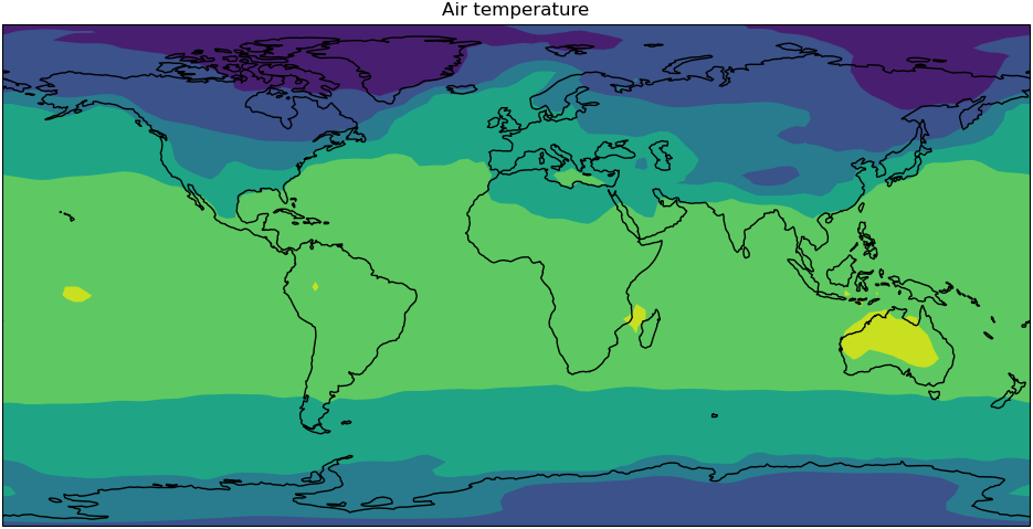
Start a session in ARE

Log in to ARE with your NCI account to start a JupyterLab session. Refer to this ARE setup guide for more details. Open the folder to your hackathon folder in nf33 where you can create a new notebook or use the Intro_to_ESMValTool.ipynb notebook in CMIP7-Hackathon\exercises\Exercise4_files.

Let’s start by importing the tool and some other tools we can use later. Note that we are importing from esmvalcore and calling it esmvaltool.

# Import the tool
import esmvalcore.experimental as esmvaltool

# Import tools for plotting
import matplotlib.pyplot as plt
import iris.quickplot

Finding a recipe

There is a utils submodule we can use to find and get recipes. Call the get_all_recipes() function to get a list of all available recipes from which you can use the find() method to return any matches. If you already know the recipe you want you can use the get_recipe() function.

In Jupyter Notebook

all_recipes = esmvaltool.get_all_recipes()
# all_recipes
all_recipes.find('python')

Get a recipe

Let’s use the examples/recipe_python.yml for this exercise, the documentation for it can be found here. Then see what’s in the recipe metadata.

Solution

example_recipe = esmvaltool.get_recipe("examples/recipe_python.yml")
example_recipe

For reading the recipe:

print(example_recipe.path.read_text())

The example_recipe here is a Recipe class with attributes data and name, see the reference.

example_recipe.name
# 'Recipe python'

Pro tip: remember the command line?

This is similar to this function in the command line whihc copies the recipe to your directory.

>esmvaltool recipes get $recipeFile

Configuration in the notebook

We can look at the default user configuration file, ~/.esmvaltool/config-user.yml by calling a CFG object as a dictionary. This gives us the ability to edit the settings. The tool can automatically download the climate data files required to run a recipe for you. You can check your download directory and output directory where your recipe runs will be saved. This CFG object is from the config module in the ESMValCore API, for more details see here.

Call the CFG object and inspect the values.

Solution

# call CFG object like this
esmvaltool.CFG

Check output directory and change

Solution

Check this location is your \scratch\nf33\$USERNAME\esmvaltool_outputs\

print(CFG['output_dir'])
# edit dir
esmvaltool.CFG['output_dir'] = '/scratch/nf33/$USERNAME/esmvaltool_outputs'

Pro tip: Missing config file or load different config

Get configuration file

Rememeber that this command line copies and creates the default user configuration file in your home .esmvaltool folder:

esmvaltool config get-config-user

Load a different configuration file to use

# an example path to other configuration file
esmvaltool.CFG.load_from_file('/home/189/fc6164/esmValTool/config-fc-copy.yml')

Running the recipe

Run the recipe and inspect the output.

Run

output = example_recipe.run()
output

This may take some time and you will see some logging messages as it runs

Inspect output

map/script1:
  ImageFile('CMIP5_bcc-csm1-1_Amon_historical_r1i1p1_tas_2000-P1M.png')
  ImageFile('CMIP6_BCC-ESM1_Amon_historical_r1i1p1f1_tas_gn_2000-P1M.png')
  DataFile('CMIP5_bcc-csm1-1_Amon_historical_r1i1p1_tas_2000-P1M.nc')
  DataFile('CMIP6_BCC-ESM1_Amon_historical_r1i1p1f1_tas_gn_2000-P1M.nc')

timeseries/script1:
  ImageFile('tas_amsterdam_CMIP5_bcc-csm1-1_Amon_historical_r1i1p1_tas_1850-2000.png')
  ImageFile('tas_amsterdam_CMIP6_BCC-ESM1_Amon_historical_r1i1p1f1_tas_gn_1850-2000.png')
  ImageFile('tas_amsterdam_MultiModelMean_historical_Amon_tas_1850-2000.png')
  ImageFile('tas_global_CMIP5_bcc-csm1-1_Amon_historical_r1i1p1_tas_1850-2000.png')
  ImageFile('tas_global_CMIP6_BCC-ESM1_Amon_historical_r1i1p1f1_tas_gn_1850-2000.png')
  DataFile('tas_amsterdam_CMIP5_bcc-csm1-1_Amon_historical_r1i1p1_tas_1850-2000.nc')
  DataFile('tas_amsterdam_CMIP6_BCC-ESM1_Amon_historical_r1i1p1f1_tas_gn_1850-2000.nc')
  DataFile('tas_amsterdam_MultiModelMean_historical_Amon_tas_1850-2000.nc')
  DataFile('tas_global_CMIP5_bcc-csm1-1_Amon_historical_r1i1p1_tas_1850-2000.nc')
  DataFile('tas_global_CMIP6_BCC-ESM1_Amon_historical_r1i1p1f1_tas_gn_1850-2000.nc')

Pro tip: run a single Diagnostic

To run a single diagnostic, the name of the task can be passed as an argument to run()

output_1 = example_recipe.run('map/script1')
output_1

Recipe output

The output can return the files as well as the image files and data files, also see the reference page.

Let’s look through this recipe output.

• Get the file paths.
• Look at one of the plots.
• Access and inspect the data used for the plots.

Solution

Print the file paths.

for result in output['map/script1']:
    print(result.path)

Look at a plot from the list of plots.

plots = [f for f in output['timeseries/script1'] if isinstance(f, esmvaltool.recipe_output.ImageFile)]
plots[-1]

Load one of the preprocessed data files.

data_files = [f for f in output['map/script1'] if isinstance(f, esmvaltool.recipe_output.DataFile)]

cube = data_files[0].load_iris()[0]
cube

Use the loaded data to make your own plot in your notebook.

Solution

# Create plot
iris.quickplot.contourf(cube)

# Set the size of the figure
plt.gcf().set_size_inches(12, 10)

# Draw coastlines
plt.gca().coastlines()

# Show the resulting figure
plt.show()

Key Points

• ESMValTool can be run in a Jupyter Notebook

• Access ImageFiles and DataFiles from the recipe run

Advanced Jupyter notebook

Overview

Teaching: 20 min
Exercises: 30 min
Compatibility:

Questions

• How to find data for ESMValTool in a Jupyter Notebook?

• How to use preprocessor functions?

Objectives

• Use the Dataset object

• Import and use preprocessor functions

• View and check the data

In this episode we will introduce the ESMValCore API in a jupyter notebook. This is reformatted from material from this blog post by Peter Kalverla. There’s also material from the example notebooks and the API reference documentation.

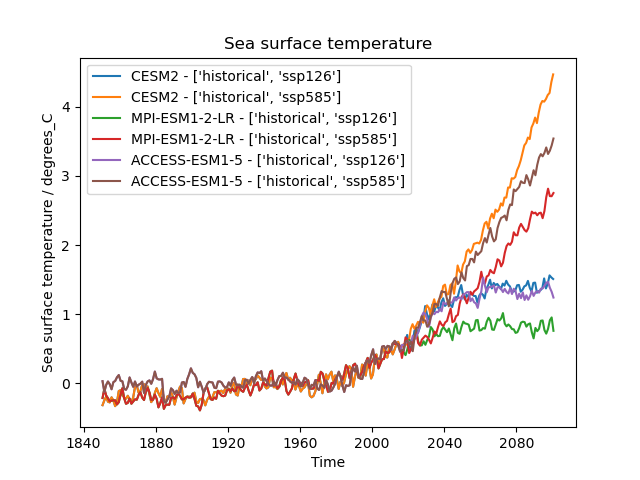
Start ARE session

Log in to ARE with your NCI account to start a JupyterLab session. Refer to this ARE setup guide for more details. Navigate to your hackathon folder /scratch/nf33/$USER/CMIP7-Hackathon/exercises/AdvancedJupyterNotebook where you can find the example_easyipcc.ipynb notebook for this exercise. Or you can create a new notebook in your workspace.

Find Datasets with facets

We have seen from running available recipes that ESMValTool is able to find data from facets that were given in the recipe. We can use this in a Notebook, including filling out the facets for data definition. To do this we will use the Dataset object from the API. Let’s look at this example.

from esmvalcore.dataset import Dataset

dataset = Dataset(
    short_name='tos',
    mip='Omon',
    project='CMIP6',
    exp='historical',
    dataset='ACCESS-ESM1-5',
    ensemble='r4i1p1f1',
    grid='gn',
)
dataset.augment_facets()
print(dataset)

Pro tip: Augmented facets in the output

When running a recipe there is a _filled recipe in the output /run folder which augments the facets.

Example recipe output folder

esmvaltool_output/flato13ipcc_figure914_CMIP6_20240729_043707/run
├── cmor_log.txt
├── fig09-14
├── flato13ipcc_figure914_CMIP6_filled.yml *
├── flato13ipcc_figure914_CMIP6.yml
├── main_log_debug.txt
├── main_log.txt
└── resource_usage.txt

Search available

Search from files locally with wildcard functionality '*' to get the available datasets.

• How can you search for all available ensembles?

Solution

dataset_search = Dataset(
    short_name='tos',
    mip='Omon',
    project='CMIP6',
    exp='historical',
    dataset='ACCESS-ESM1-5',
    ensemble='*',
    grid='gn',
)
ensemble_datasets = list(dataset_search.from_files())

print([ds['ensemble'] for ds in ensemble_datasets])

There is also the ability to search on ESGF nodes and download. See reference for more details.

Add supplementary variables

Supplementary variables can be added to the Dataset object which can be used for certain preprocessors such as area statistics and weighting.

• Add the area file to this Dataset.

Solution

# Discard augmented facets as they will be different for areacello
dataset = Dataset(**dataset.minimal_facets)

# Add areacello as supplementary dataset
dataset.add_supplementary(short_name='areacello', mip='Ofx')

# Autocomplete and inspect
dataset.augment_facets()
print(dataset.summary())

Loading the data and inspect

# Before load, checks location of file
print(dataset.files)

cube = dataset.load()
cube

Output

sea_surface_temperature / (degC)          (time: 1980; cell index along second dimension: 300; cell index along first dimension: 360)
    Dimension coordinates:
        time                                   x                                        -                                      -
        cell index along second dimension      -                                        x                                      -
        cell index along first dimension       -                                        -                                      x
    Auxiliary coordinates:
        latitude                               -                                        x                                      x
        longitude                              -                                        x                                      x
    Cell measures:
        cell_area                              -                                        x                                      x
    Cell methods:
        0                                 area: mean where sea
        1                                 time: mean
    Attributes:
        Conventions                       'CF-1.7 CMIP-6.2'
        activity_id                       'CMIP'
        branch_method                     'standard'
        branch_time_in_child              0.0
        branch_time_in_parent             -594980
        cmor_version                      '3.4.0'
        data_specs_version                '01.00.30'
        experiment                        'all-forcing simulation of the recent past'
        experiment_id                     'historical'
        external_variables                'areacello'
        forcing_index                     1
        frequency                         'mon'
        further_info_url                  'https://furtherinfo.es-doc.org/CMIP6.CSIRO.ACCESS-ESM1-5.historical.no ...'
        grid                              'native atmosphere N96 grid (145x192 latxlon)'
        grid_label                        'gn'
        initialization_index              1
        institution                       'Commonwealth Scientific and Industrial Research Organisation, Aspendale, ...'
        institution_id                    'CSIRO'
        license                           'CMIP6 model data produced by CSIRO is licensed under a Creative Commons ...'
        mip_era                           'CMIP6'
        nominal_resolution                '250 km'
        notes                             "Exp: ESM-historical; Local ID: HI-08; Variable: tos (['sst'])"
        parent_activity_id                'CMIP'
        parent_experiment_id              'piControl'
        parent_mip_era                    'CMIP6'
        parent_source_id                  'ACCESS-ESM1-5'
        parent_time_units                 'days since 1850-1-1 00:00:00'
        parent_variant_label              'r1i1p1f1'
        physics_index                     1
        product                           'model-output'
        realization_index                 4
        realm                             'ocean'
        run_variant                       'forcing: GHG, Oz, SA, Sl, Vl, BC, OC, (GHG = CO2, N2O, CH4, CFC11, CFC12, ...'
        source                            'ACCESS-ESM1.5 (2019): \naerosol: CLASSIC (v1.0)\natmos: HadGAM2 (r1.1, ...'
        source_id                         'ACCESS-ESM1-5'
        source_type                       'AOGCM'
        sub_experiment                    'none'
        sub_experiment_id                 'none'
        table_id                          'Omon'
        table_info                        'Creation Date:(30 April 2019) MD5:40e9ef53d4d2ec9daef980b76f23d39a'
        title                             'ACCESS-ESM1-5 output prepared for CMIP6'
        variable_id                       'tos'
        variant_label                     'r4i1p1f1'
        version                           'v20200529'

Preprocessors

As mentioned in previous lessons, the idea of preprocessors are that they are a set of functions that can be applied in a centralised, documented and efficient way. There are a broad range of operations that are commonly done to input data before diagnostics or metrics are applied and can be done to all the datasets in a recipe consistently. See the documentation to read further.

Exercise: apply preprocessors using the API

See API reference to check the arguments for preprocessor functions. For this exercise, find;

1. The global mean,
2. Then anomalies which we can get monthly,
3. Then aggregate annually for plotting and inspect the cube.

Solution

from esmvalcore.preprocessor import annual_statistics, anomalies, area_statistics

# Set the reference period for anomalies 
reference_period = {
    "start_year": 1950, "start_month": 1, "start_day": 1,
    "end_year": 1979, "end_month": 12, "end_day": 31,
}

cube = area_statistics(cube, operator='mean')
cube = anomalies(cube, reference=reference_period, period='month')
cube = annual_statistics(cube, operator='mean')
cube.convert_units('degrees_C')
cube

sea_surface_temperature / (degrees_C)     (time: 165)
    Dimension coordinates:
        time                                   x
    Auxiliary coordinates:
        year                                   x
    Scalar coordinates:
        cell index along first dimension  179, bound=(0, 359)
        cell index along second dimension 149, bound=(0, 299)
        latitude                          6.0 degrees_north, bound=(-78.0, 90.0) degrees_north
        longitude                         179.9867706298828 degrees_east, bound=(0.0, 359.9735412597656) degrees_east
    Cell methods:
        0                                 area: mean where sea
        1                                 time: mean
        2                                 latitude: longitude: mean
        3                                 year: mean

Plot data

Iris has wrappers for matplotlib to plot the processed cubes. This is useful in a notebook to help develop your recipe with the esmvalcore preprocessors.

from iris import quickplot
quickplot.plot(cube)

Custom code

We have so far solely used ESMValCore, however, you can use your own custom code and being in a Notebook means you can try straight away. Now, continue with other libraries and make custom plots such as xarray.

import xarray as xr
da = xr.DataArray.from_iris(cube)
da.plot()
print(da)

Build workflow and diagnostic

Exercise - Easy IPCC plot for sea surface temperature

Let’s pull some of these bits together to build a diagnostic.

• Using the Dataset object, make a template which we can use to find multiple datasets we want to analyse together for variable tos.
• The datasets being "CESM2", "MPI-ESM1-2-LR", "ACCESS-ESM1-5" and experiments 'ssp126', 'ssp585' with historical, iterate to build a list of datasets.
• Apply the preprocessors to each dataset and plot the result

Solution

import cf_units
import matplotlib.pyplot as plt
from iris import quickplot

from esmvalcore.config import CFG
from esmvalcore.dataset import Dataset
from esmvalcore.preprocessor import annual_statistics, anomalies, area_statistics


# Settings for automatic ESGF search
CFG['search_esgf'] = 'when_missing'

# Declare common dataset facets
template = Dataset(
    short_name='tos',
    mip='Omon',
    project='CMIP6',
    exp= '*', # We'll fill this below
    dataset='*',  # We'll fill this below
    ensemble='r4i1p1f1',
    grid='gn',
)

# Substitute data sources and experiments
datasets = []
for dataset_id in ["CESM2", "MPI-ESM1-2-LR", "ACCESS-ESM1-5"]:
    for experiment_id in ['ssp126', 'ssp585']:
        dataset = template.copy(dataset=dataset_id, exp=['historical', experiment_id])
        dataset.add_supplementary(short_name='areacello', mip='Ofx', exp='historical')
        dataset.augment_facets()
        datasets.append(dataset)

# Set the reference period for anomalies 
reference_period = {
    "start_year": 1950, "start_month": 1, "start_day": 1,
    "end_year": 1979, "end_month": 12, "end_day": 31,
}

# (Down)load, pre-process, and plot the cubes
for dataset in datasets: 
    cube = dataset.load()
    cube = area_statistics(cube, operator='mean')
    cube = anomalies(cube, reference=reference_period, period='month')  # notice 'month'
    cube = annual_statistics(cube, operator='mean')
    cube.convert_units('degrees_C')

    # Make sure all datasets use the same calendar for plotting
    tcoord = cube.coord('time')
    tcoord.units = cf_units.Unit(tcoord.units.origin, calendar='gregorian')

    # Plot
    quickplot.plot(cube, label=f"{dataset['dataset']} - {dataset['exp']}")

# Show the plot
plt.legend()
plt.show()

Pro tip: Convert to recipe

We can use the helper to start making the recipe. A recipe can be used for reproducibility of an analysis. This list the datasets in a recipe format and we would then have to create the preprocessors and diagnostic script.

from esmvalcore.dataset import datasets_to_recipe
import yaml

for dataset in datasets:
    dataset.facets['diagnostic'] = 'easy_ipcc'
print(yaml.safe_dump(datasets_to_recipe(datasets)))

Output

datasets:
- dataset: ACCESS-ESM1-5
  exp:
  - historical
  - ssp126
- dataset: ACCESS-ESM1-5
  exp:
  - historical
  - ssp585
- dataset: CESM2
  exp:
  - historical
  - ssp126
- dataset: CESM2
  exp:
  - historical
  - ssp585
- dataset: MPI-ESM1-2-LR
  exp:
  - historical
  - ssp126
- dataset: MPI-ESM1-2-LR
  exp:
  - historical
  - ssp585
diagnostics:
  easy_ipcc:
    variables:
      tos:
        ensemble: r4i1p1f1
        grid: gn
        mip: Omon
        project: CMIP6
        supplementary_variables:
        - exp: historical
          mip: Ofx
          short_name: areacello
        timerange: 1850/2100

Run through Minimal example notebook

Partly shown in the introduction episode. Find the example in your cloned hackathon folder: CMIP7-Hackathon\exercises\IntroductionESMValTool\Minimal_example.ipynb This notebook includes:

• Plot 2D field on a map
• Hovmoller Diagram
• Wind speed over Australia
• Air Potential Temperature (3D data) Transect
• Australian mean temperature timeseries

Exercise: Sea-ice area

Use observation data and 2 model datasets to show trends in sea-ice.

• Using variable siconc which is a fraction percent(0-100)
• Using datasets:
  • dataset:'ACCESS-ESM1-5', exp:'historical', ensemble:'r1i1p1f1', timerange:'1960/2010'
  • dataset :'ACCESS-OM2', exp:'omip2', ensemble='r1i1p1f1', timerange:'0306/0366'
• Using observations:
  • dataset:'NSIDC-G02202-sh', tier:'3', version:'4', timerange:'1979/2018'

1. Extract Southern hemisphere
2. Use only valid values (15 -100 %)
3. Sum sea ice area which will be the fraction multiplied by cell area and summed
4. Plot yearly minimum and maximum value

Solution notebook - CMIP7-Hackathon/exercises/AdvancedJupyterNotebook/example_seaicearea.ipynb

1. Define datasets:

from esmvalcore.dataset import Dataset
obs = Dataset(
    short_name='siconc', mip='SImon', project='OBS6', type='reanaly',
    dataset='NSIDC-G02202-sh', tier='3', version='4', timerange='1979/2018',
)
# Add areacello as supplementary dataset
obs.add_supplementary(short_name='areacello', mip='Ofx')

model = Dataset(
    short_name='siconc', mip='SImon', project='CMIP6', activity='CMIP',
    dataset='ACCESS-ESM1-5', ensemble='r1i1p1f1', grid='gn', exp='historical',
    timerange='1960/2010', institute = '*',
)

om_facets={'dataset' :'ACCESS-OM2', 'exp':'omip2', 'activity':'OMIP', 'timerange':'0306/0366' }

model.add_supplementary(short_name='areacello', mip='Ofx')

model_om = model.copy(**om_facets) 

Tip: Check dataset files can be found

The observational dataset used is a Tier 3, so with some licensing restrictions. It is not directly accesible here. Check files can be found for all the datasets:

for ds in [model, model_om, obs]:
    print(ds['dataset'],' : ' ,ds.files)
    print(ds.supplementaries[0].files)

This observation dataset does have a downloader and formatter with ESMValTool, you can use these data functions mentioned in the supported data lesson:

esmvaltool data download --config_file <path to config-user.yml>  NSIDC-G02202-sh
esmvaltool data format --config_file <path to config-user.yml>  NSIDC-G02202-sh

For this plot we can drop it for now. But you can also try to find and add another dataset. eg:

obs_other = Dataset(
    short_name='siconc', mip='*', project='OBS', type='*',
    dataset='*', tier='*', timerange='1979/2018'
)
obs_other.files

2. Use esmvalcore API preprocessors on the datasets and plot results

import iris
import matplotlib.pyplot as plt
from iris import quickplot
from esmvalcore.preprocessor import (
            mask_outside_range,
            extract_region,
            area_statistics,
            annual_statistics
)
# om - at index 1 to offset years
# drop observations that cannot be found
load_data = [model, model_om] #, obs] 

# function to use for both min and max ['max','min'] 

def trends_seaicearea(min_max):
    plt.clf()
    for i,data in enumerate(load_data):
        cube = data.load()
        cube = mask_outside_range(cube, 15, 100)
        cube = extract_region(cube,0,360,-90,0)
        cube = area_statistics(cube, 'sum')
        cube = annual_statistics(cube, min_max)
    
        iris.util.promote_aux_coord_to_dim_coord(cube, 'year')
        cube.convert_units('km2')
        if i == 1: ## om years 306/366 apply offset
            cube.coord('year').points = [y + 1652 for y in cube.coord('year').points]
        label_name = data['dataset']
        print(label_name, cube.shape)
        quickplot.plot(cube, label=label_name)
    
    plt.title(f'Trends in Sea-Ice {min_max.title()}ima')
    plt.ylabel('Sea-Ice Area (km2)')
    plt.legend()

trends_seaicearea('min')

Key Points

• API can be used as a helper to develop recipes

• Preprocessors can be used in a Jupyter Notebook to check the output

• Use datasets_to_recipe helper to start making recipes

Running the ILAMB on Gadi

Overview

Teaching: 30 min
Exercises: 60 min
Compatibility:

Questions

• How do I run the ILAMB on NCI GADI?

Objectives

• Understand how to load, configure and run the ILAMB using the ACCESS-NRI ILAMB-Workflow

What is the ILAMB?

The International Land Model Benchmarking (ILAMB) project is a model-data intercomparison and integration project designed to improve the performance of land models and, in parallel, improve the design of new measurement campaigns to reduce uncertainties associated with key land surface processes.

The purpose of the Quickstart Guide is to provide users of GADI with a streamlined process to rapidly run the International Land Model Benchmarking (ILAMB) system. ACCESS-NRI offers an already configured ILAMB module via the ILAMB-Workflow, enabling users to quickly initiate benchmarking tasks without the need for deployment. This guide is designed to help users efficiently begin evaluating land model outputs against observational datasets with minimal setup time.

How to cite the ILAMB?

Collier, N., Hoffman, F. M., Lawrence, D. M., Keppel-Aleks, G., Koven, C. D., Riley, W. J., et al. (2018). The International Land Model Benchmarking (ILAMB) system: Design, theory, and implementation. Journal of Advances in Modeling Earth Systems, 10, 2731–2754. https://doi.org/10.1029/2018MS001354

The ILAMB on NCI-Gadi

For NCI users, ACCESS-NRI is providing a conda environment with the latest version of ILAMB through project xp65..

module use /g/data/xp65/public/modules
module load ilamb-workflow

or

module use /g/data/xp65/public/modules
module load conda/access-med

To run the ILAMB, you need to execute the command ilamb-run with a number of arguments/files:

ilamb-run --config config.cfg --model_setup model_setup.txt --regions global

• config.cfg defines which observables and observational datasets will be compared
• model_setup.txt defines the paths of the models that will be compared

Below we explain how to setup the necessary directory structures and the example files mentioned above. For detailed information on the arguments of ilamb-run, please consult the official ILAMB documentation.

Organising Data and Model Outputs for ILAMB Benchmarking

ILAMB requires files to be organized within a specific directory structure, consisting of DATA and MODELS directories. The DATA directory contains observational datasets, while the MODELS directory holds the output from the models you wish to benchmark. Adhering to this structure is essential for ILAMB to correctly locate and compare the datasets during the benchmarking process.

The following directory tree represents a typical ILAMB_ROOT setup for CMIP comparison on NCI/Gadi:

$ILAMB_ROOT/
|-- DATA -> /g/data/ct11/access-nri/replicas/ILAMB
|-- MODELS
  |-- ACCESS-ESM1-5
  |   `-- piControl
  |       `-- r3i1p1f1
                 ├── evspsbl.nc
                 ├── hfds.nc
                 ├── hfls.nc
                 ├── hfss.nc
                 ├── hurs.nc
                 ├── pr.nc
                 ├── rlds.nc
                 ├── rlus.nc
                 ├── rsds.nc
                 ├── rsus.nc
                 ├── tasmax.nc
                 ├── tasmin.nc
                 ├── tas.nc
                 └── tsl.nc

The top level of this directory structure is defined by the ILAMB_ROOT path, which should be set as an environment variable:

export ILAMB_ROOT=/path/to/your/ILAMB_ROOT/directory

By exporting this path as $ILAMB_ROOT, you ensure that the ILAMB can correctly locate the necessary directories and files during the benchmarking process.”

1. the DATA directory: this is where we keep the observational datasets each in a subdirectory bearing the name of the variable.
2. the MODEL directory: this directory can be populated with symbolic links to the model outputs.

Automating ILAMB Directory Structure Setup with ilamb-tree-generator

To simplify the setup of an ILAMB-ROOT directory tree, ACCESS-NRI offers a tool called ilamb-tree-generator, available within the ILAMB-Workflow through the access-med environment of the xp65 project.

The ilamb-tree-generator automates the creation of the necessary ILAMB directory structure. It efficiently generates symlinks to the ACCESS-NRI Replicated Datasets for Climate Model Evaluation and to the relevant sections of the model outputs. This automation helps ensure that your ILAMB benchmarking setup is correctly configured with minimal manual intervention.

To add model outputs, you can list them in a YAML file, formatted as follows:

datasets:
   - {mip: CMIP, institute: CSIRO-ARCCSS, dataset: ACCESS-CM2, project: CMIP6, exp: piControl, ensemble: r3i1p1f1}
   - {mip: CMIP, institute: CSIRO-ARCCSS, dataset: ACCESS-CM2, project: CMIP6, exp: piControl, ensemble: r3i1p2f1}
   - {mip: CMIP, institute: CSIRO-ARCCSS, dataset: ACCESS-CM2, project: CMIP6, exp: piControl, ensemble: r3i1p3f1}

Once your YAML file is ready, you can run the tool from the command line to generate the directory structure:

ilamb-tree-generator --datasets models.yml --ilamb_root $ILAMB_ROOT

This command will automatically create the appropriate folders under the specified ILAMB_ROOT path, ensuring that your data is organized correctly for ILAMB benchmarking.”

Exercise

Copy the above to a models.yml file and try to run the ilamb-tree-generator

ILAMB model selection: model_setup.txt

In the model_setup.txt, you can select all the model outputs that you want to compare.

Assuming you want to compare the three models that we used in ILAMB_ROOT/MODELS, you would need to create a model_setup.txt file wehere you define both the model labels and their paths:

 # Model Name (used as label), ABSOLUTE/PATH/TO/MODELS or relative to $ILAMB_ROOT/ , Time Shift
   piControl_r3i1p1f1, /scratch/nf33/yz9299/ILAMB-sep-2024/ILAMB_ROOT/MODELS/ACCESS-CM2/piControl/r3i1p1f1/, 1000, 1920
   piControl_r3i1p2f1, /scratch/nf33/yz9299/ILAMB-sep-2024/ILAMB_ROOT/MODELS/ACCESS-CM2/piControl/r3i1p2f1/, 1000, 1920
   piControl_r3i1p3f1, /scratch/nf33/yz9299/ILAMB-sep-2024/ILAMB_ROOT/MODELS/ACCESS-CM2/piControl/r3i1p3f1/, 1000, 1920

Since ILAMB require model-output data and observational data should have time overlap. In this case, our piControl data time-range is (1000-1080) , and most of the observational data time range is (1900-2000), so we specify time shift in model_setup.txt from 1000 to 1920, make it comparable with observational data.

Configuring and Running a Benchmark Study with the ILAMB

ILAMB uses a config.cfg file as its configuration file to initiate a benchmark study. This file allows you to set up comparison sections and specify which variables from which datasets will be compared.

An example configuration file for ILAMB on Gadi might be named config.cfg. It could be used to compare your models with two variables from the radiation and energy cycle, as measured by the Clouds and the Earth’s Radiant Energy System (CERES) project:

This configuration file is used to define the comparison sections, variables, and observational datasets required for running ILAMB on Gadi. The file is organised with the following structure:

[h1:] Sections
[h2:] Variables
[]    Observational Datasets

• Sections: Define the major comparison categories or groups within the benchmark study.
• Variables: Specify the particular variables that will be compared between model outputs and observational data.
• Observational Datasets: List the datasets used for comparison, detailing where ILAMB will source the observational data.

For further guidance on how to create and use configuration files, refer to the ILAMB Tutorial on Configure Files. You can also consult the ILAMB and IOMB dataset collections at ILAMB Datasets.

A minimal Example

[h1: Hydrology Cycle]
bgcolor = "#E6F9FF"

[h2: Evapotranspiration]
variable       = "et"
alternate_vars = "evspsbl"
cmap           = "Blues"
weight         = 5
mass_weighting = True

[MODIS]
source        = "DATA/evspsbl/MODIS/et_0.5x0.5.nc"
weight        = 15
table_unit    = "mm d-1"
plot_unit     = "mm d-1"
relationships = "Precipitation/GPCPv2.3","SurfaceAirTemperature/CRU4.02"

this example configuration file is set up for running ILAMB on Gadi and specifies details for comparing data related to the hydrology cycle. Here’s a breakdown of what each section does:

 [h1: Hydrology Cycle]
 bgcolor = "#E6F9FF"

• [h1: Hydrology Cycle]: This section defines a major comparison category called “Hydrology Cycle” and sets a background color for visualizations.

 [h2: Evapotranspiration]
 variable       = "et"
 alternate_vars = "evspsbl"
 cmap           = "Blues"
 weight         = 5
 mass_weighting = True

• [h2: Evapotranspiration]: This subsection focuses on “Evapotranspiration” within the hydrology cycle.
  • variable: Specifies the main variable to compare, which is “et” (evapotranspiration).
  • alternate_vars: Provides an alternate variable name “evspsbl” that might be used in the data.
  • cmap: Sets the color map for plotting the data, here using shades of blue.
  • weight: Assigns a weight of 5 to this variable in the comparisons.
  • mass_weighting: Indicates that mass weighting should be applied (True).

 [MODIS]
 source        = "DATA/evspsbl/MODIS/et_0.5x0.5.nc"
 weight        = 15
 table_unit    = "mm d-1"
 plot_unit     = "mm d-1"
 relationships = "Precipitation/GPCPv2.3","SurfaceAirTemperature/CRU4.02"

• [MODIS]: This section specifies details for the observational dataset related to MODIS.
  • source: Points to the file location of the MODIS dataset.
  • weight: Assigns a weight of 15 to this dataset in the comparisons.
  • table_unit: Defines the unit of measurement for the dataset, “mm d-1” (millimeters per day).
  • plot_unit: Specifies the unit of measurement for plotting, also “mm d-1”.
  • relationships: Lists other related datasets, such as precipitation and surface air temperature, indicating how they relate to the MODIS dataset.

Exercise: Adding a Second Observational Dataset to the ILAMB Configuration File

In this exercise, you will add a second observational dataset to your ILAMB configuration file. Follow these steps to integrate a new dataset, [MOD16A2], into your existing configuration:

1. Open Your ILAMB Configuration File: Locate and open the ILAMB configuration file you are currently using.

2. Identify the Section for Observational Datasets:
   • Scroll to the section of the file where observational datasets are listed.
3. Add the New Dataset:
   • Insert the following block of code to include the [MOD16A2] observational dataset:

    [MOD16A2]
    source        = "DATA/evspsbl/MOD16A2/et.nc"
    weight        = 15
    table_unit    = "mm d-1"
    plot_unit     = "mm d-1"
    relationships = "Precipitation/GPCPv2.3","SurfaceAirTemperature/CRU4.02"
   

   • This entry specifies the details for the new dataset:
     • source: Path to the dataset file.
     • weight: Weight assigned to this dataset for comparisons.
     • table_unit: Unit of measurement used in tables.
     • plot_unit: Unit of measurement used in plots.
     • relationships: Lists other related datasets for comparison.
4. Save Your Changes: Make sure to save the configuration file after adding the new dataset.

Solution

# This configure file specifies comparison sections, variables and observational data for running ILAMB on Gadi.

# See https://www.ilamb.org/doc/first_steps.html#configure-files for the ILAMB Tutorial that addesses Configure Files
# See https://www.ilamb.org/datasets.html for the ILAMB and IOMB collections

# Structure:
# [h1:] Sections
# [h2:] Variables
# []    Observational Datasets

#=======================================================================================

[h1: Hydrology Cycle]
bgcolor = "#E6F9FF"

[h2: Evapotranspiration]
variable       = "et"
alternate_vars = "evspsbl"
cmap           = "Blues"
weight         = 5
mass_weighting = True

[MODIS]
source        = "DATA/evspsbl/MODIS/et_0.5x0.5.nc"
weight        = 15
table_unit    = "mm d-1"
plot_unit     = "mm d-1"
relationships = "Precipitation/GPCPv2.3","SurfaceAirTemperature/CRU4.02"

[MOD16A2]
source        = "DATA/evspsbl/MOD16A2/et.nc"
weight        = 15
table_unit    = "mm d-1"
plot_unit     = "mm d-1"
relationships = "Precipitation/GPCPv2.3","SurfaceAirTemperature/CRU4.02"


#~~~~~~~~~~~~~~~~~~~~~~~~~~~~~~~~~~~~~~~~~~~~~~~~~~~~~~~~~~~~~~~~~~~~~~~~~~

Exercise: Adding New Comparison Details to the ILAMB Configuration File

In this exercise, you will add a new section for “Latent Heat” to the ILAMB configuration file. Follow the steps below:

1. Open your existing ILAMB configuration file: Locate and open the configuration file you have been working with.

2. Add a new subsection for Latent Heat:
   • Scroll to the appropriate location in the file where you want to add the new details.
   • Insert the following content to define the “Latent Heat” comparison:

    [h2: Latent Heat]
    variable       = "hfls"
    alternate_vars = "le"
    cmap           = "Oranges"
    weight         = 5
    mass_weighting = True
   

   • This section sets up a comparison for “Latent Heat,” specifying the variable, alternate names, color map, weight, and mass weighting.
3. Add details for the FLUXCOM dataset:
   • Below the “Latent Heat” subsection, add the following content to define the FLUXCOM dataset:

    [FLUXCOM]
    source   = "DATA/hfls/FLUXCOM/le.nc"
    land     = True
    weight   = 9
    skip_iav = True
   

   • This section specifies the source file for the FLUXCOM dataset, assigns a weight, indicates whether land data is included, and whether to skip inter-annual variability.
4. Save your changes: Ensure that the file is saved with the new sections included.

Solution

# This configure file specifies comparison sections, variables and observational data for running ILAMB on Gadi.

# See https://www.ilamb.org/doc/first_steps.html#configure-files for the ILAMB Tutorial that addesses Configure Files
# See https://www.ilamb.org/datasets.html for the ILAMB and IOMB collections

# Structure:
# [h1:] Sections
# [h2:] Variables
# []    Observational Datasets

#=======================================================================================

[h1: Hydrology Cycle]
bgcolor = "#E6F9FF"

[h2: Evapotranspiration]
variable       = "et"
alternate_vars = "evspsbl"
cmap           = "Blues"
weight         = 5
mass_weighting = True

[MODIS]
source        = "DATA/evspsbl/MODIS/et_0.5x0.5.nc"
weight        = 15
table_unit    = "mm d-1"
plot_unit     = "mm d-1"
relationships = "Precipitation/GPCPv2.3","SurfaceAirTemperature/CRU4.02"

[MOD16A2]
source        = "DATA/evspsbl/MOD16A2/et.nc"
weight        = 15
table_unit    = "mm d-1"
plot_unit     = "mm d-1"
relationships = "Precipitation/GPCPv2.3","SurfaceAirTemperature/CRU4.02"


#~~~~~~~~~~~~~~~~~~~~~~~~~~~~~~~~~~~~~~~~~~~~~~~~~~~~~~~~~~~~~~~~~~~~~~~~~~

[h2: Latent Heat]
variable       = "hfls"
alternate_vars = "le"
cmap           = "Oranges"
weight         = 5
mass_weighting = True

[FLUXCOM]
source   = "DATA/hfls/FLUXCOM/le.nc"
land     = True
weight   = 9
skip_iav = True

#~~~~~~~~~~~~~~~~~~~~~~~~~~~~~~~~~~~~~~~~~~~~~~~~~~~~~~~~~~~~~~~~~~~~~~~~~~

A Comprehensive example

# This configure file specifies comparison sections, variables and observational data for running ILAMB on Gadi.

# See https://www.ilamb.org/doc/first_steps.html#configure-files for the ILAMB Tutorial that addesses Configure Files
# See https://www.ilamb.org/datasets.html for the ILAMB and IOMB collections

# Structure:
# [h1:] Sections
# [h2:] Variables
# []    Observational Datasets

#=======================================================================================

[h1: Hydrology Cycle]
bgcolor = "#E6F9FF"

[h2: Evapotranspiration]
variable       = "et"
alternate_vars = "evspsbl"
cmap           = "Blues"
weight         = 5
mass_weighting = True

[MODIS]
source        = "DATA/evspsbl/MODIS/et_0.5x0.5.nc"
weight        = 15
table_unit    = "mm d-1"
plot_unit     = "mm d-1"
relationships = "Precipitation/GPCPv2.3","SurfaceAirTemperature/CRU4.02"

[MOD16A2]
source        = "DATA/evspsbl/MOD16A2/et.nc"
weight        = 15
table_unit    = "mm d-1"
plot_unit     = "mm d-1"
relationships = "Precipitation/GPCPv2.3","SurfaceAirTemperature/CRU4.02"


#~~~~~~~~~~~~~~~~~~~~~~~~~~~~~~~~~~~~~~~~~~~~~~~~~~~~~~~~~~~~~~~~~~~~~~~~~~

[h2: Latent Heat]
variable       = "hfls"
alternate_vars = "le"
cmap           = "Oranges"
weight         = 5
mass_weighting = True

[FLUXCOM]
source   = "DATA/hfls/FLUXCOM/le.nc"
land     = True
weight   = 9
skip_iav = True

[DOLCE]
source   = "DATA/evspsbl/DOLCE/DOLCE.nc"
weight   = 15
land     = True

#~~~~~~~~~~~~~~~~~~~~~~~~~~~~~~~~~~~~~~~~~~~~~~~~~~~~~~~~~~~~~~~~~~~~~~~~~~

[h2: Sensible Heat]
variable       = "hfss"
alternate_vars = "sh"
weight         = 2
mass_weighting = True

[FLUXCOM]
source   = "DATA/hfss/FLUXCOM/sh.nc"
weight   = 15
skip_iav = True

###########################################################################

[h1: Radiation and Energy Cycle]
bgcolor = "#FFECE6"

#~~~~~~~~~~~~~~~~~~~~~~~~~~~~~~~~~~~~~~~~~~~~~~~~~~~~~~~~~~~~~~~~~~~~~~~~~~

[h2: Albedo]
variable = "albedo"
weight   = 1
ctype    = "ConfAlbedo"

[CERESed4.1]
source   = "DATA/albedo/CERESed4.1/albedo.nc"
weight   = 20

[GEWEX.SRB]
source   = "DATA/albedo/GEWEX.SRB/albedo_0.5x0.5.nc"
weight   = 20

#~~~~~~~~~~~~~~~~~~~~~~~~~~~~~~~~~~~~~~~~~~~~~~~~~~~~~~~~~~~~~~~~~~~~~~~~~~

[h2: Surface Upward SW Radiation]
variable = "rsus"
weight   = 1

[FLUXNET2015]
source   = "DATA/rsus/FLUXNET2015/rsus.nc"
weight   = 12

[GEWEX.SRB]
source   = "DATA/rsus/GEWEX.SRB/rsus_0.5x0.5.nc"
weight   = 15

[WRMC.BSRN]
source   = "DATA/rsus/WRMC.BSRN/rsus.nc"
weight   = 12

#~~~~~~~~~~~~~~~~~~~~~~~~~~~~~~~~~~~~~~~~~~~~~~~~~~~~~~~~~~~~~~~~~~~~~~~~~~

[h2: Surface Net SW Radiation]
variable = "rsns"
derived  = "rsds-rsus"
weight   = 1

[CERESed4.1]
source   = "DATA/rsns/CERESed4.1/rsns.nc"
weight   = 15

[FLUXNET2015]
source   = "DATA/rsns/FLUXNET2015/rsns.nc"
weight   = 12

[GEWEX.SRB]
source   = "DATA/rsns/GEWEX.SRB/rsns_0.5x0.5.nc"
weight   = 15

[WRMC.BSRN]
source   = "DATA/rsns/WRMC.BSRN/rsns.nc"
weight   = 12

#~~~~~~~~~~~~~~~~~~~~~~~~~~~~~~~~~~~~~~~~~~~~~~~~~~~~~~~~~~~~~~~~~~~~~~~~~~

[h2: Surface Upward LW Radiation]
variable = "rlus"
weight   = 1

[FLUXNET2015]
source   = "DATA/rlus/FLUXNET2015/rlus.nc"
weight   = 12

[GEWEX.SRB]
source   = "DATA/rlus/GEWEX.SRB/rlus_0.5x0.5.nc"
weight   = 15

[WRMC.BSRN]
source   = "DATA/rlus/WRMC.BSRN/rlus.nc"
weight   = 12

#~~~~~~~~~~~~~~~~~~~~~~~~~~~~~~~~~~~~~~~~~~~~~~~~~~~~~~~~~~~~~~~~~~~~~~~~~~

[h2: Surface Net LW Radiation]
variable = "rlns"
derived  = "rlds-rlus"
weight   = 1

[CERESed4.1]
source   = "DATA/rlns/CERESed4.1/rlns.nc"
weight   = 15 

[FLUXNET2015]
source   = "DATA/rlns/FLUXNET2015/rlns.nc"
weight   = 12

[GEWEX.SRB]
source   = "DATA/rlns/GEWEX.SRB/rlns_0.5x0.5.nc"
weight   = 15

[WRMC.BSRN]
source   = "DATA/rlns/WRMC.BSRN/rlns.nc"
weight   = 12

#~~~~~~~~~~~~~~~~~~~~~~~~~~~~~~~~~~~~~~~~~~~~~~~~~~~~~~~~~~~~~~~~~~~~~~~~~~

[h2: Surface Net Radiation]
variable = "rns"
derived  = "rlds-rlus+rsds-rsus"
weight = 2

[CERESed4.1]
source   = "DATA/rns/CERESed4.1/rns.nc"
weight   = 15

[FLUXNET2015]
source   = "DATA/rns/FLUXNET2015/rns.nc"
weight   = 12

[GEWEX.SRB]
source   = "DATA/rns/GEWEX.SRB/rns_0.5x0.5.nc"
weight   = 15

[WRMC.BSRN]
source   = "DATA/rns/WRMC.BSRN/rns.nc"
weight   = 12

###########################################################################

[h1: Forcings]
bgcolor = "#EDEDED"

#~~~~~~~~~~~~~~~~~~~~~~~~~~~~~~~~~~~~~~~~~~~~~~~~~~~~~~~~~~~~~~~~~~~~~~~~~~

[h2: Surface Air Temperature]
variable = "tas"
weight   = 2

[FLUXNET2015]
source   = "DATA/tas/FLUXNET2015/tas.nc"
weight   = 9

#~~~~~~~~~~~~~~~~~~~~~~~~~~~~~~~~~~~~~~~~~~~~~~~~~~~~~~~~~~~~~~~~~~~~~~~~~~

[h2: Diurnal Temperature Range]
variable = "dtr"
weight   = 2
derived  = "tasmax-tasmin"

[CRU4.02]
source   = "DATA/dtr/CRU4.02/dtr.nc"
weight   = 25

#~~~~~~~~~~~~~~~~~~~~~~~~~~~~~~~~~~~~~~~~~~~~~~~~~~~~~~~~~~~~~~~~~~~~~~~~~~

[h2: Precipitation]
variable       = "pr"
cmap           = "Blues"
weight         = 2
mass_weighting = True

[FLUXNET2015]
source     = "DATA/pr/FLUXNET2015/pr.nc"
land       = True
weight     = 9
table_unit = "mm d-1"
plot_unit  = "mm d-1"

[GPCCv2018]
source     = "DATA/pr/GPCCv2018/pr.nc"
land       = True
weight     = 20
table_unit = "mm d-1"
plot_unit  = "mm d-1"
space_mean = True

[GPCPv2.3]
source     = "DATA/pr/GPCPv2.3/pr.nc"
land       = True
weight     = 20
table_unit = "mm d-1"
plot_unit  = "mm d-1"
space_mean = True

#~~~~~~~~~~~~~~~~~~~~~~~~~~~~~~~~~~~~~~~~~~~~~~~~~~~~~~~~~~~~~~~~~~~~~~~~~~

[h2: Surface Relative Humidity]
variable       = "rhums"
alternate_vars = "hurs"
cmap           = "Blues"
weight         = 3
mass_weighting = True

[CRU4.02]
source     = "DATA/rhums/CRU4.02/rhums.nc"
weight     = 10

#~~~~~~~~~~~~~~~~~~~~~~~~~~~~~~~~~~~~~~~~~~~~~~~~~~~~~~~~~~~~~~~~~~~~~~~~~~

[h2: Surface Downward SW Radiation]
variable = "rsds"
weight   = 2

[FLUXNET2015]
source   = "DATA/rsds/FLUXNET2015/rsds.nc"
weight   = 12

[GEWEX.SRB]
source   = "DATA/rsds/GEWEX.SRB/rsds_0.5x0.5.nc"
weight   = 15

[WRMC.BSRN]
source   = "DATA/rsds/WRMC.BSRN/rsds.nc"
weight   = 12

#~~~~~~~~~~~~~~~~~~~~~~~~~~~~~~~~~~~~~~~~~~~~~~~~~~~~~~~~~~~~~~~~~~~~~~~~~~

[h2: Surface Downward LW Radiation]
variable = "rlds"
weight   = 1

[FLUXNET2015]
source   = "DATA/rlds/FLUXNET2015/rlds.nc"
weight   = 12

[GEWEX.SRB]
source   = "DATA/rlds/GEWEX.SRB/rlds_0.5x0.5.nc"
weight   = 15

[WRMC.BSRN]
source   = "DATA/rlds/WRMC.BSRN/rlds.nc"
weight   = 12

Running the ILAMB

Now that we have the configuration file set up, you can run the study using the ilamb-run script via the aforementioned

ilamb-run --config config.cfg --model_setup model_setup.txt --regions global

Taking advantage of multiprocessors

Because of the computational costs, you need to run ILAMB through a Portable Batch System (PBS) job on Gadi.

The following default PBS file, let’s call it ilamb_test.job, can help you to setup your own, while making sure to use the correct project (#PBS -P) to charge your computing cost to:

 #!/bin/bash
 
 #PBS -N ilamb_test
 #PBS -l wd
 #PBS -P your_compute_project_here
 #PBS -q normalbw
 #PBS -l walltime=0:20:00  
 #PBS -l ncpus=14
 #PBS -l mem=63GB           
 #PBS -l jobfs=10GB        
 #PBS -l storage=gdata/ct11+gdata/hh5+gdata/xp65+gdata/fs38+gdata/oi10+gdata/zv30
 
 # ILAMB is provided through projects xp65. We will use the latter here
 module use /g/data/xp65/public/modules
 module load conda/access-med
 
 # Define the ILAMB Path, expecting it to be where you start this job from
 export ILAMB_ROOT=./
 export CARTOPY_DATA_DIR=/g/data/xp65/public/apps/cartopy-data
 
 # Run ILAMB in parallel with the config.cfg configure file for the models defined in model_setup.txt
 mpiexec -n 10 ilamb-run --config config.cfg --model_setup model_setup.txt --regions global

You should adjust this file to your own specifications (including the storage access to your models). Save the file in the $ILAMB_ROOT and submit its job to the queue from there via

qsub ilamb_test.job

Running this job will create a _build directory with the comparison results within $ILAMB_ROOT. You can adjust the place of this directory via a agrument --build_dir argument for ilamb-run.

View Result

Once you finish your ILAMB run, you will get your ILAMB result. The default path to the result is ./_built，unless you specified --build_dir before you run your experiment with ILAMB.

Use VSCode to Simplily Visualise

This is the recommended way to visualise result, you need to install extension Live Server in your VSCode, Type live server into the extensions search bar and select the Live Server extension published by Ritwick Dey marked with the red ellipse below. This extension allows us to preview html files from a browser on our computer, and will update automatically as the html file is updated in VS Code. We will use this extension to preview some of the ESMValTool recipe outputs that come in html format. Click install to add the extension.

Once you installed the extension, go to your result directory and right click index.html, choose Open with Live Server, then you will have your result opened in your browser.

In case you don’t use VSCode or Live Server doesn’t work for you, this is another way to view the result. You change your directory to the result directory, create a new local host by below command:

python3 -m http.server

Your ILAMB result can be viewed in the following address: localhost address:

http://0.0.0.0:8000/

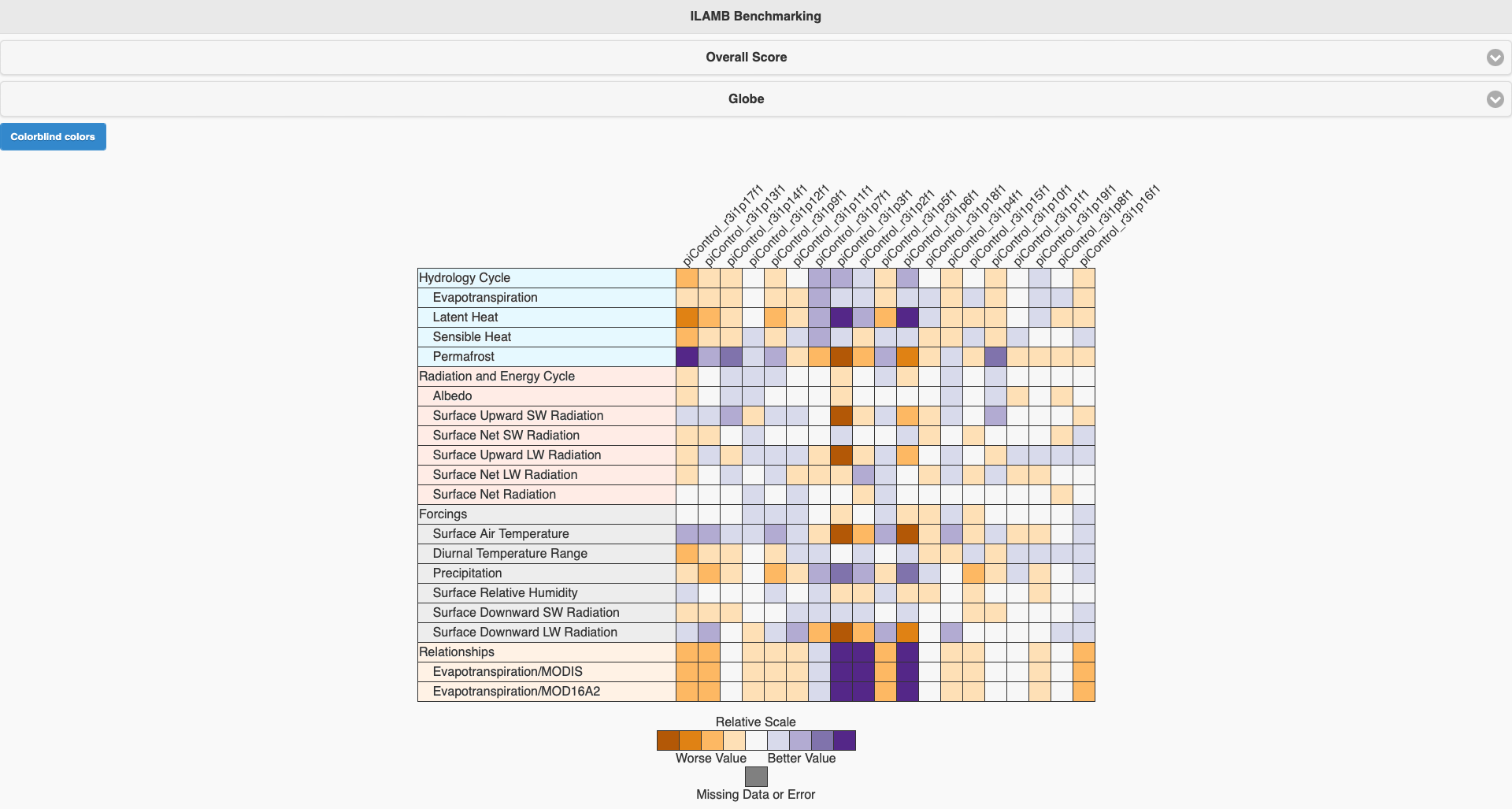
This is an example that we compared different ensemble members in piControl use the config.cfg we showed above. Click each raw, you can see the detail of conparison result with each observational data.

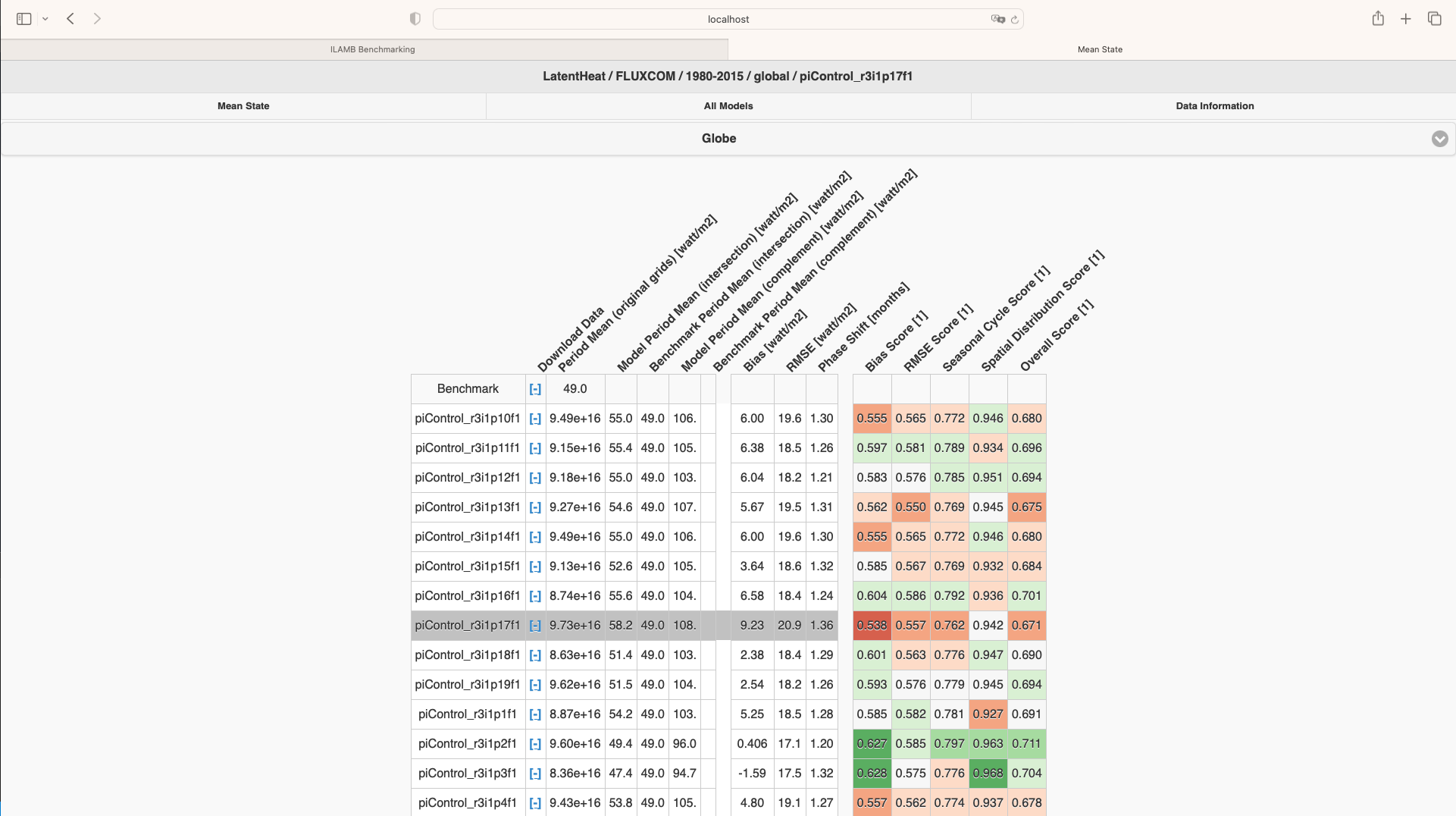
Click each raw of this matrix, you can view all the graphs of comparison results of this specific dataset.

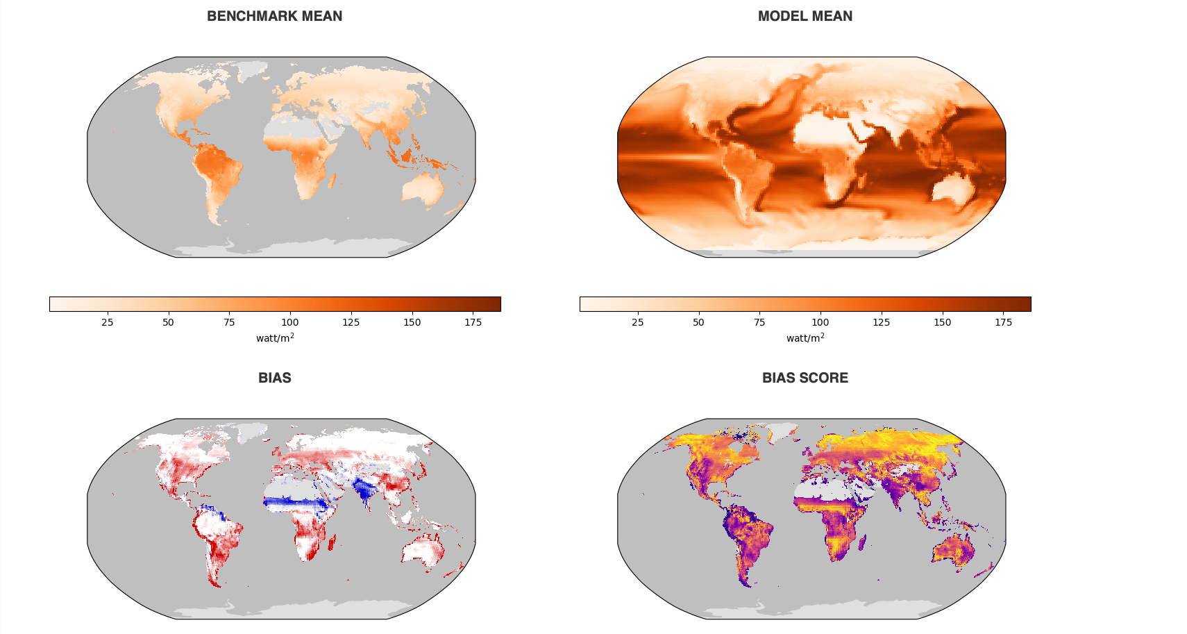
And also if you would like to view all graphs of one specific comparasion, you can click All Models, and choose which comparison you would liek to see(use Temporally integrated period mean rmse score as example), then you will get then all togather.

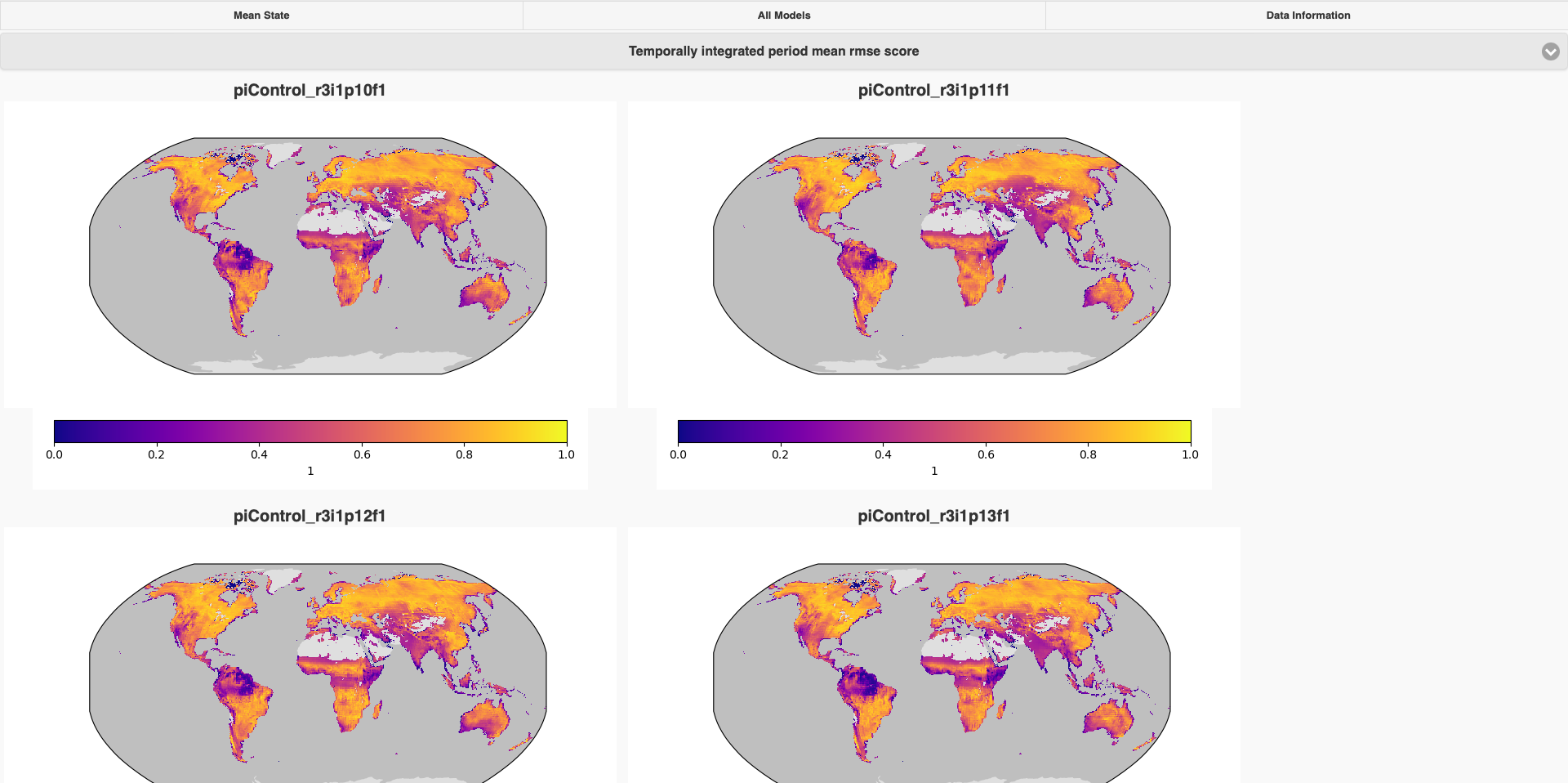
Key Points

• The ACCESS-NRI ILAMB-Workflow facilitates the configuration of the ILAMB on NCI Gadi.

• Users need to set up a run using a configuration file.

• The ilamb-tree-generator allows to quickly build a data directory srtucture for the ILAMB.

• The ILAMB can take advantage of the multiple CPUs available on Gadi.

ILAMB support for RAW ACCESS-ESM outputs

Overview

Teaching: 15 min
Exercises: 15 min
Compatibility:

Questions

• What do we mean by CMORising?

• How to use ilamb-tree-generator to CMORise Raw Access data

Objectives

• Analyse raw (non-CMORised) ACCESS outputs with the ILAMB

In this episode we will introduce how to use ilamb-tree-generator as a CMORiser to help you use ILAMB to evaluate Access raw output. But before that, we will introduce what is ‘CMORise’ first.

What is CMORisation?

“CMORise” refers to the process of converting climate model output data into a standardized format that conforms to the Climate and Forecast (CF) metadata conventions. This process involves using the Climate Model Output Rewriter (CMOR) tool, which ensures that the data adheres to specific requirements for structure, metadata, and units, making it easier to compare and share across different climate models.

Use ilamb-tree-generator to CMORise Access raw output

Load the ILAMB-Workflow module

Theilamb-tree-generator is available in the ILAMB-Workflow module that can be loaded as follow:

module use /g/data/xp65/public/modules
module load ilamb-workflow

or

module use /g/data/xp65/public/modules
module load conda/access-med

Configuring Dataset Inputs for ilamb-tree-generator: CMIP and Non-CMIP Examples”

As mentioned earlier, the ilamb-tree-generator utilizes a .yml file for all input configurations. This format is consistent for different datasets. Below is an example configuration for both CMIP and non-CMIP datasets:

datasets:
    - {mip: CMIP, institute: CSIRO, dataset: ACCESS-ESM1-5, project: CMIP6, exp: historical, ensemble: r1i1p1f1}
    - {mip: non-CMIP, institute: CSIRO, dataset: ACCESS-ESM1-5, project: CMIP6, exp: HI-CN-05}

The first entry represents a CMIP dataset, which is the standard usage for ilamb-tree-generator. The second entry corresponds to an ACCESS raw output, which is a non-CMIP dataset. Although most parameters are similar, there are specific settings for non-CMIP datasets. Here are the details of each parameter:

• mip: Set to non-CMIP to activate the CMORiser for non-CMIP data.
• path: For users working with their own ACCESS raw data, specify the root directory here. If not provided, the tool will default to using data in the p73 directory.

run ilamb-tree-generator

After setting up the config.yml file, run the ilamb-tree-generator. This will generate the CMORized data within the ILAMB-ROOT directory, making it accessible for ILAMB to read and use:

ilamb-tree-generator --datasets {your-config.yml-file} --ilamb_root $ILAMB_ROOT

Once it finish, you will get your CMORised data been stored by variable names in this format:

.
├── DATA
└── MODELS
    └── ACCESS-ESM1-5
        └── HI-CN-05
            ├── cSoil.nc
            ├── cVeg.nc
            ├── evspsbl.nc
            ├── gpp.nc
            ├── hfls.nc
            ├── hfss.nc
            ├── hurs.nc
            ├── lai.nc
            ├── nbp.nc
            ├── pr.nc
            ├── ra.nc
            ├── rh.nc
            ├── rlds.nc
            ├── rlus.nc
            ├── rsds.nc
            ├── rsus.nc
            ├── tasmax.nc
            ├── tasmin.nc
            ├── tas.nc
            └── tsl.nc

Limitations

ilamb-tree-generator doesn’t support all variable in ACCESS-ESM1-5, only 19 variables which is required in ilamb.cfg. Will try to add more variables in the next version.

Key Points

• The ILAMB-Workflow only support RAW ACCESS data

• Running the ILAMB-Workflow on RAW ACCESS data can take some time. Consider if it is appropriate for your work

• Only a limited number of CMIP variables are supported