Advanced Jupyter notebook
Overview
Teaching: 20 min
Exercises: 30 min
Compatibility: ESMValTool v2.11.0Questions
How to find data for ESMValTool in a Jupyter Notebook?
How to use preprocessor functions?
Objectives
Use the Dataset object
Import and use preprocessor functions
View and check the data
In this episode we will introduce the ESMValCore API in a jupyter notebook. This is reformatted from material from
this blog post
by Peter Kalverla. There’s also material from the example notebooks and the
API reference documentation.
Start ARE session
Log in to ARE with your NCI account to start a JupyterLab session.
Refer to this ARE setup guide for more details.
Navigate to your hackathon folder /scratch/nf33/$USER/CMIP7-Hackathon/exercises/AdvancedJupyterNotebook
where you can find the example_easyipcc.ipynb notebook for this exercise.
Or you can create a new notebook in your workspace.
Find Datasets with facets
We have seen from running available recipes that ESMValTool is able to find data from facets that were given in
the recipe. We can use this in a Notebook, including filling out the facets for data definition.
To do this we will use the Dataset object from the API. Let’s look at this example.
from esmvalcore.dataset import Dataset

dataset = Dataset(
    short_name='tos',
    mip='Omon',
    project='CMIP6',
    exp='historical',
    dataset='ACCESS-ESM1-5',
    ensemble='r4i1p1f1',
    grid='gn',
)
dataset.augment_facets()
print(dataset)
Pro tip: Augmented facets in the output
When running a recipe there is a
_filledrecipe in the output /run folder which augments the facets.Example recipe output folder
esmvaltool_output/flato13ipcc_figure914_CMIP6_20240729_043707/run
├── cmor_log.txt
├── fig09-14
├── flato13ipcc_figure914_CMIP6_filled.yml *
├── flato13ipcc_figure914_CMIP6.yml
├── main_log_debug.txt
├── main_log.txt
└── resource_usage.txt
Search available
Search from files locally with wildcard functionality
'*'to get the available datasets.
- How can you search for all available ensembles?
Solution
dataset_search = Dataset(
    short_name='tos',
    mip='Omon',
    project='CMIP6',
    exp='historical',
    dataset='ACCESS-ESM1-5',
    ensemble='*',
    grid='gn',
)
ensemble_datasets = list(dataset_search.from_files())

print([ds['ensemble'] for ds in ensemble_datasets])
There is also the ability to search on ESGF nodes and download. See reference for more details.
Add supplementary variables
Supplementary variables can be added to the
Datasetobject which can be used for certain preprocessors such as area statistics and weighting.
- Add the area file to this Dataset.
Solution
# Discard augmented facets as they will be different for areacello
dataset = Dataset(**dataset.minimal_facets)

# Add areacello as supplementary dataset
dataset.add_supplementary(short_name='areacello', mip='Ofx')

# Autocomplete and inspect
dataset.augment_facets()
print(dataset.summary())
Loading the data and inspect
# Before load, checks location of file
print(dataset.files)

cube = dataset.load()
cube
Output
sea_surface_temperature / (degC)          (time: 1980; cell index along second dimension: 300; cell index along first dimension: 360)
    Dimension coordinates:
        time                                   x                                        -                                      -
        cell index along second dimension      -                                        x                                      -
        cell index along first dimension       -                                        -                                      x
    Auxiliary coordinates:
        latitude                               -                                        x                                      x
        longitude                              -                                        x                                      x
    Cell measures:
        cell_area                              -                                        x                                      x
    Cell methods:
        0                                 area: mean where sea
        1                                 time: mean
    Attributes:
        Conventions                       'CF-1.7 CMIP-6.2'
        activity_id                       'CMIP'
        branch_method                     'standard'
        branch_time_in_child              0.0
        branch_time_in_parent             -594980
        cmor_version                      '3.4.0'
        data_specs_version                '01.00.30'
        experiment                        'all-forcing simulation of the recent past'
        experiment_id                     'historical'
        external_variables                'areacello'
        forcing_index                     1
        frequency                         'mon'
        further_info_url                  'https://furtherinfo.es-doc.org/CMIP6.CSIRO.ACCESS-ESM1-5.historical.no ...'
        grid                              'native atmosphere N96 grid (145x192 latxlon)'
        grid_label                        'gn'
        initialization_index              1
        institution                       'Commonwealth Scientific and Industrial Research Organisation, Aspendale, ...'
        institution_id                    'CSIRO'
        license                           'CMIP6 model data produced by CSIRO is licensed under a Creative Commons ...'
        mip_era                           'CMIP6'
        nominal_resolution                '250 km'
        notes                             "Exp: ESM-historical; Local ID: HI-08; Variable: tos (['sst'])"
        parent_activity_id                'CMIP'
        parent_experiment_id              'piControl'
        parent_mip_era                    'CMIP6'
        parent_source_id                  'ACCESS-ESM1-5'
        parent_time_units                 'days since 1850-1-1 00:00:00'
        parent_variant_label              'r1i1p1f1'
        physics_index                     1
        product                           'model-output'
        realization_index                 4
        realm                             'ocean'
        run_variant                       'forcing: GHG, Oz, SA, Sl, Vl, BC, OC, (GHG = CO2, N2O, CH4, CFC11, CFC12, ...'
        source                            'ACCESS-ESM1.5 (2019): \naerosol: CLASSIC (v1.0)\natmos: HadGAM2 (r1.1, ...'
        source_id                         'ACCESS-ESM1-5'
        source_type                       'AOGCM'
        sub_experiment                    'none'
        sub_experiment_id                 'none'
        table_id                          'Omon'
        table_info                        'Creation Date:(30 April 2019) MD5:40e9ef53d4d2ec9daef980b76f23d39a'
        title                             'ACCESS-ESM1-5 output prepared for CMIP6'
        variable_id                       'tos'
        variant_label                     'r4i1p1f1'
        version                           'v20200529'
Preprocessors
As mentioned in previous lessons, the idea of preprocessors are that they are a set of functions that can be applied in a centralised, documented and efficient way. There are a broad range of operations that are commonly done to input data before diagnostics or metrics are applied and can be done to all the datasets in a recipe consistently. See the documentation to read further.
Exercise: apply preprocessors using the API
See API reference to check the arguments for preprocessor functions. For this exercise, find;
- The global mean,
- Then anomalies which we can get monthly,
- Then aggregate annually for plotting and inspect the cube.
Solution
from esmvalcore.preprocessor import annual_statistics, anomalies, area_statistics

# Set the reference period for anomalies
reference_period = {
    "start_year": 1950, "start_month": 1, "start_day": 1,
    "end_year": 1979, "end_month": 12, "end_day": 31,
}

cube = area_statistics(cube, operator='mean')
cube = anomalies(cube, reference=reference_period, period='month')
cube = annual_statistics(cube, operator='mean')
cube.convert_units('degrees_C')
cube
sea_surface_temperature / (degrees_C) (time: 165) Dimension coordinates: time x Auxiliary coordinates: year x Scalar coordinates: cell index along first dimension 179, bound=(0, 359) cell index along second dimension 149, bound=(0, 299) latitude 6.0 degrees_north, bound=(-78.0, 90.0) degrees_north longitude 179.9867706298828 degrees_east, bound=(0.0, 359.9735412597656) degrees_east Cell methods: 0 area: mean where sea 1 time: mean 2 latitude: longitude: mean 3 year: mean
Plot data
Iris has wrappers for matplotlib to plot the processed cubes. This is useful in a notebook to help develop your recipe with the esmvalcore preprocessors.
from iris import quickplot
quickplot.plot(cube)
Custom code
We have so far solely used ESMValCore, however, you can use your own custom code and
being in a Notebook means you can try straight away. Now, continue with other libraries
and make custom plots such as xarray.
import xarray as xr
da = xr.DataArray.from_iris(cube)
da.plot()
print(da)
Build workflow and diagnostic
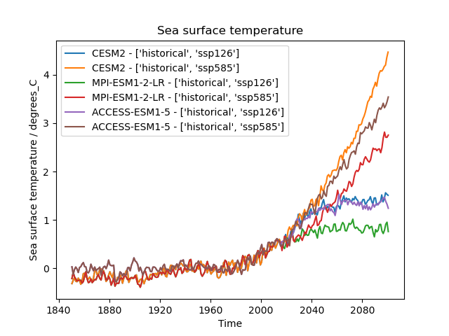
Exercise - Easy IPCC plot for sea surface temperature
Let’s pull some of these bits together to build a diagnostic.
- Using the
Datasetobject, make a template which we can use to find multiple datasets we want to analyse together for variabletos.- The datasets being
"CESM2", "MPI-ESM1-2-LR", "ACCESS-ESM1-5"and experiments'ssp126', 'ssp585'with historical, iterate to build a list of datasets.- Apply the preprocessors to each dataset and plot the result
Solution
import cf_units
import matplotlib.pyplot as plt
from iris import quickplot

from esmvalcore.config import CFG
from esmvalcore.dataset import Dataset
from esmvalcore.preprocessor import annual_statistics, anomalies, area_statistics


# Settings for automatic ESGF search
CFG['search_esgf'] = 'when_missing'

# Declare common dataset facets
template = Dataset(
    short_name='tos',
    mip='Omon',
    project='CMIP6',
    exp= '*', # We'll fill this below
    dataset='*',  # We'll fill this below
    ensemble='r4i1p1f1',
    grid='gn',
)

# Substitute data sources and experiments
datasets = []
for dataset_id in ["CESM2", "MPI-ESM1-2-LR", "ACCESS-ESM1-5"]:
    for experiment_id in ['ssp126', 'ssp585']:
        dataset = template.copy(dataset=dataset_id, exp=['historical', experiment_id])
        dataset.add_supplementary(short_name='areacello', mip='Ofx', exp='historical')
        dataset.augment_facets()
        datasets.append(dataset)

# Set the reference period for anomalies
reference_period = {
    "start_year": 1950, "start_month": 1, "start_day": 1,
    "end_year": 1979, "end_month": 12, "end_day": 31,
}

# (Down)load, pre-process, and plot the cubes
for dataset in datasets:
    cube = dataset.load()
    cube = area_statistics(cube, operator='mean')
    cube = anomalies(cube, reference=reference_period, period='month')  # notice 'month'
    cube = annual_statistics(cube, operator='mean')
    cube.convert_units('degrees_C')

    # Make sure all datasets use the same calendar for plotting
    tcoord = cube.coord('time')
    tcoord.units = cf_units.Unit(tcoord.units.origin, calendar='gregorian')

    # Plot
    quickplot.plot(cube, label=f"{dataset['dataset']} - {dataset['exp']}")

# Show the plot
plt.legend()
plt.show()
Pro tip: Convert to recipe
We can use the helper to start making the recipe. A recipe can be used for reproducibility of an analysis. This list the datasets in a recipe format and we would then have to create the preprocessors and diagnostic script.
from esmvalcore.dataset import datasets_to_recipe
import yaml

for dataset in datasets:
    dataset.facets['diagnostic'] = 'easy_ipcc'
print(yaml.safe_dump(datasets_to_recipe(datasets)))
Output
datasets:
- dataset: ACCESS-ESM1-5
  exp:
  - historical
  - ssp126
- dataset: ACCESS-ESM1-5
  exp:
  - historical
  - ssp585
- dataset: CESM2
  exp:
  - historical
  - ssp126
- dataset: CESM2
  exp:
  - historical
  - ssp585
- dataset: MPI-ESM1-2-LR
  exp:
  - historical
  - ssp126
- dataset: MPI-ESM1-2-LR
  exp:
  - historical
  - ssp585
diagnostics:
  easy_ipcc:
    variables:
      tos:
        ensemble: r4i1p1f1
        grid: gn
        mip: Omon
        project: CMIP6
        supplementary_variables:
        - exp: historical
          mip: Ofx
          short_name: areacello
        timerange: 1850/2100
Run through Minimal example notebook
Partly shown in the introduction episode. Find the example in your cloned hackathon folder:
CMIP7-Hackathon\exercises\IntroductionESMValTool\Minimal_example.ipynbThis notebook includes:
- Plot 2D field on a map
- Hovmoller Diagram
- Wind speed over Australia
- Air Potential Temperature (3D data) Transect
- Australian mean temperature timeseries
Exercise: Sea-ice area
Use observation data and 2 model datasets to show trends in sea-ice.
- Using variable
siconcwhich is a fraction percent(0-100)- Using datasets:
dataset:'ACCESS-ESM1-5', exp:'historical', ensemble:'r1i1p1f1', timerange:'1960/2010'dataset :'ACCESS-OM2', exp:'omip2', ensemble='r1i1p1f1', timerange:'0306/0366'- Using observations:
dataset:'NSIDC-G02202-sh', tier:'3', version:'4', timerange:'1979/2018'
- Extract Southern hemisphere
- Use only valid values (15 -100 %)
- Sum sea ice area which will be the fraction multiplied by cell area and summed
- Plot yearly minimum and maximum value
Solution notebook -
CMIP7-Hackathon/exercises/AdvancedJupyterNotebook/example_seaicearea.ipynb1. Define datasets:
from esmvalcore.dataset import Dataset
obs = Dataset(
    short_name='siconc', mip='SImon', project='OBS6', type='reanaly',
    dataset='NSIDC-G02202-sh', tier='3', version='4', timerange='1979/2018',
)
# Add areacello as supplementary dataset
obs.add_supplementary(short_name='areacello', mip='Ofx')

model = Dataset(
    short_name='siconc', mip='SImon', project='CMIP6', activity='CMIP',
    dataset='ACCESS-ESM1-5', ensemble='r1i1p1f1', grid='gn', exp='historical',
    timerange='1960/2010', institute = '*',
)

om_facets={'dataset' :'ACCESS-OM2', 'exp':'omip2', 'activity':'OMIP', 'timerange':'0306/0366' }

model.add_supplementary(short_name='areacello', mip='Ofx')

model_om = model.copy(**om_facets)
Tip: Check dataset files can be found
The observational dataset used is a Tier 3, so with some licensing restrictions. It is not directly accesible here. Check files can be found for all the datasets:
for ds in [model, model_om, obs]:
    print(ds['dataset'],' : ' ,ds.files)
    print(ds.supplementaries[0].files)
This observation dataset does have a downloader and formatter with ESMValTool, you can use these data functions mentioned in the supported data lesson:
esmvaltool data download --config_file <path to config-user.yml>  NSIDC-G02202-sh
esmvaltool data format --config_file <path to config-user.yml>  NSIDC-G02202-sh
For this plot we can drop it for now. But you can also try to find and add another dataset. eg:
obs_other = Dataset(
    short_name='siconc', mip='*', project='OBS', type='*',
    dataset='*', tier='*', timerange='1979/2018'
)
obs_other.files
2. Use esmvalcore API preprocessors on the datasets and plot results
import iris
import matplotlib.pyplot as plt
from iris import quickplot
from esmvalcore.preprocessor import (
            mask_outside_range,
            extract_region,
            area_statistics,
            annual_statistics
)
# om - at index 1 to offset years
# drop observations that cannot be found
load_data = [model, model_om] #, obs]

# function to use for both min and max ['max','min']

def trends_seaicearea(min_max):
    plt.clf()
    for i,data in enumerate(load_data):
        cube = data.load()
        cube = mask_outside_range(cube, 15, 100)
        cube = extract_region(cube,0,360,-90,0)
        cube = area_statistics(cube, 'sum')
        cube = annual_statistics(cube, min_max)

        iris.util.promote_aux_coord_to_dim_coord(cube, 'year')
        cube.convert_units('km2')
        if i == 1: ## om years 306/366 apply offset
            cube.coord('year').points = [y + 1652 for y in cube.coord('year').points]
        label_name = data['dataset']
        print(label_name, cube.shape)
        quickplot.plot(cube, label=label_name)

    plt.title(f'Trends in Sea-Ice {min_max.title()}ima')
    plt.ylabel('Sea-Ice Area (km2)')
    plt.legend()

trends_seaicearea('min')
Key Points
API can be used as a helper to develop recipes
Preprocessors can be used in a Jupyter Notebook to check the output
Use
datasets_to_recipehelper to start making recipes